- Introduction
- 1. Introduction to Quantitative Analysis
- 2. Descriptive Statistics
- 3. T-test for Difference in Means and Hypothesis Testing
- 4. Bivariate linear regression models
- 5. Multiple linear regression models
- 6. Assumptions and Violations of Assumptions
- 7. Interactions
- 8. Panel Data, Time-Series Cross-Section Models
- 9. Binary models: Logit
- 10. Frequently Asked Questions
- 11. Optional Material
- 12. Datasets
- 13. R Resources
- 14. References
- Published with GitBook
9. Binary models: Logit
9.2 Solutions
Exercise 1
Estimate a model similar to model 2 in the seminar and add Civic Duty (CivicDutyScores) and party identification (PartyID). Show and discuss descriptive statistics of the variables in a meaningful way. E.g.: what does a unit change in a variable mean, are the variables comparable. Do this for all variables but concentrate your discussion on the interesting ones.
Solution
We begin by clearing our workspace. Loading all the packages we need and then reloading the data set. We only keep the variables we care about. Furthermore, we remove missings. This can be done within the select function. R knows that we are working with the data set bes because we initialized with the line bes <- bes %>%. Therefore, we just write na.omit(). You can use the same approach to drop missings on certain variables only, e.g. na.omit(turnout) would drop missings from the turnout variable.
# clearing workspace
rm(list = ls())

# loading packages we need
library(Zelig) # load BEFORE dplyr!!!
library(foreign) # to load .dta files
library(lmtest) # for likelihood ratio test
library(texreg) # regression tables
Warning: package 'texreg' was built under R version 3.2.3
library(dplyr) # data manipulation/ summary statistics

# load data
bes <- read.dta("http://uclspp.github.io/PUBLG100/data/bes.dta")

# selecting variables we need
bes <- bes %>%
  select(turnout = Turnout,
         income = Income,
         age = Age,
         male = Gender,
         partyid = PartyID,
         influence = Influence,
         civicduty = CivicDutyScores,
         polinfoindex,
         edu15,
         edu16,
         edu17,
         edu18,
         edu19plus,
         in_school,
         in_uni) %>%
  na.omit()

# check if there are missings left
summary(bes)
    turnout           income            age             male
 Min.   :0.0000   Min.   : 1.000   Min.   :18.00   Min.   :0.0000
 1st Qu.:0.0000   1st Qu.: 4.000   1st Qu.:37.00   1st Qu.:0.0000
 Median :1.0000   Median : 5.000   Median :50.00   Median :0.0000
 Mean   :0.7407   Mean   : 5.322   Mean   :50.92   Mean   :0.4424
 3rd Qu.:1.0000   3rd Qu.: 7.000   3rd Qu.:65.00   3rd Qu.:1.0000
 Max.   :1.0000   Max.   :13.000   Max.   :99.00   Max.   :1.0000
    partyid        influence        civicduty         polinfoindex
 Min.   :0.000   Min.   : 1.000   Min.   :-3.51592   Min.   :0.000
 1st Qu.:0.000   1st Qu.: 1.000   1st Qu.:-0.66407   1st Qu.:4.000
 Median :1.000   Median : 3.000   Median : 0.20109   Median :6.000
 Mean   :0.596   Mean   : 3.609   Mean   :-0.04343   Mean   :5.409
 3rd Qu.:1.000   3rd Qu.: 5.000   3rd Qu.: 0.67849   3rd Qu.:7.000
 Max.   :1.000   Max.   :11.000   Max.   : 2.69098   Max.   :8.000
     edu15            edu16            edu17             edu18
 Min.   :0.0000   Min.   :0.0000   Min.   :0.00000   Min.   :0.000
 1st Qu.:0.0000   1st Qu.:0.0000   1st Qu.:0.00000   1st Qu.:0.000
 Median :0.0000   Median :0.0000   Median :0.00000   Median :0.000
 Mean   :0.3331   Mean   :0.2588   Mean   :0.09012   Mean   :0.087
 3rd Qu.:1.0000   3rd Qu.:1.0000   3rd Qu.:0.00000   3rd Qu.:0.000
 Max.   :1.0000   Max.   :1.0000   Max.   :1.00000   Max.   :1.000
   edu19plus        in_school             in_uni
 Min.   :0.0000   Min.   :-0.405100   Min.   :0.0000
 1st Qu.:0.0000   1st Qu.: 0.000000   1st Qu.:0.0000
 Median :0.0000   Median : 0.000000   Median :0.0000
 Mean   :0.2057   Mean   : 0.008061   Mean   :0.0173
 3rd Qu.:0.0000   3rd Qu.: 0.000000   3rd Qu.:0.0000
 Max.   :1.0000   Max.   : 1.000000   Max.   :1.0000
# frequency table
table(bes$partyid)
   0    1
1681 2480
# histogram
hist(bes$civicduty, main = "Distribution of Civic Duty",
     xlab = "Level of Civic Duty (larger values more feeling of duty)",
     ylab = "Frequency")
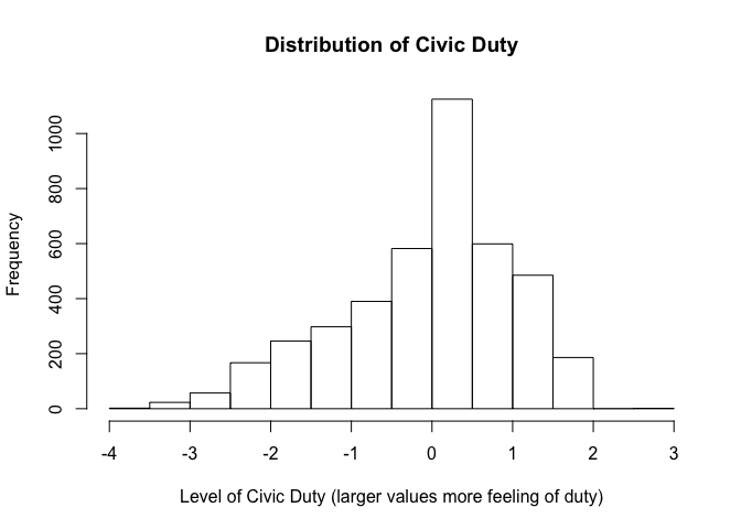
The summary function tells us that civicduty is a continuous variable. It ranges from a minimum of -3.5 to a maximum of 2.7, has an average value of 0 and is slightly left-skewed. A 'one-unit-change' in civic duty corresponds to a hefty 16% percentage point change in the sense of duty (1/(-3.5 - 2.7)). That means a one-unit-change in civic duty is a lot.
partyid is binary, 60% of the respondents feel attached to a political party. A unit increase in partyid corresponds to a change from a person who does not identify with a political party to someone who does. Thus, the variable captures two distinct groups of people.
As the two independent variables (civicduty and partyid) are not on the same scale - the former ranges from -3.5 to 2.7 and the latter takes only two values: 0 or 1 - the coefficient sizes will not be directly comparable. That means we cannot say which has a bigger effect just by looking at the absolute size of the coefficients. You can only compare effect sizes of different coefficients when variables are on the same scale (if you are interested, have a look at Stock & Watson Chapter 2.4 to see how to standardize variables and make them comparable)
The resource theory claims that people turn out to vote when they possess more material and cognitive resources. The corresponding variables are income and polinfoindex.
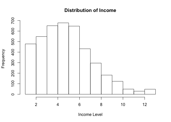
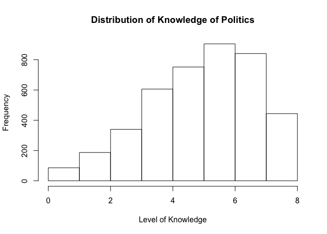
income is interval scaled with a minimum of 1 (poorest) and a maximum of 13 (richest). Average income is 5.3. The variable is heavily left-skewed, meaning that there are many more poorer than richer people. polinfoindex measures knowledge about politics and ranges from 0 (fewest) to 8 (most). The mean is 5.4 and the distribution is right-skewed, fewer people have little knowledge than have a lot. For both variables the theoretical range corresponds to the range observed in the sample. A one-unit-change in income corresponds to 8% of the range of income. A one-unit-change in knowledge about politics corresponds to 13% of the range of the variable.
# histogram Income
hist(bes$income, main = "Distribution of Income",
     xlab = "Income Level",
     ylab = "Frequency")
# histogram polinfoindex
hist(bes$polinfoindex, main = "Distribution of Knowledge of Politics",
     xlab = "Level of Knowledge",
     ylab = "Frequency",
     breaks = seq(0, 8, 1))
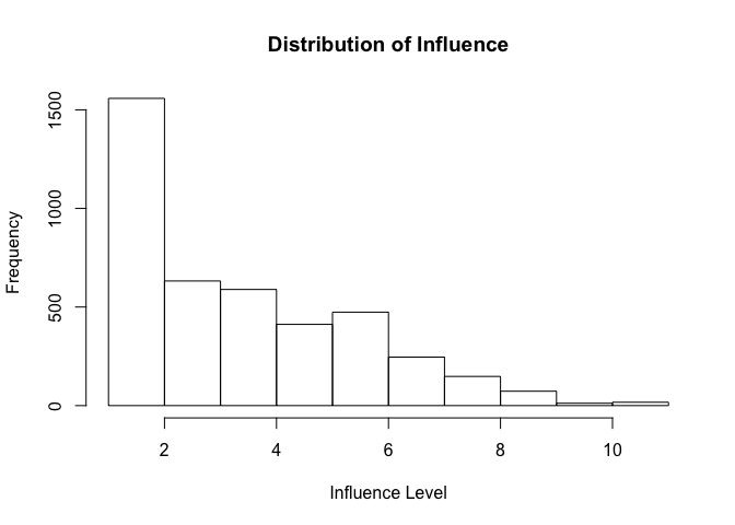
influence measures the subjective feeling that one can influence politics. The range is from 1 to 11. The average value is 3.61. The distribution is heavily left-skewed reflecting that most people feel they have little influence over politics. A unit increase corresponds to 10% of the range of the variable.
# histogram influence
hist(bes$influence, main = "Distribution of Influence",
     xlab = "Influence Level",
     ylab = "Frequency")
Education, gender and age are socioeconomic controls (we do not really care about them but excluding them could lead to omitted variable bias). The modal category of education is 15 years of schooling (33%), the average age is 51 and 44% of respondents are male.
Our dependent variable is turnout, 74% of respondents reported that they turned out to vote. Considering actual participation rates, this value seems rather high and suggests some bias in reporting the result that is socially desirable. 74% sets the baseline for our model. We need to correctly categorize more than 74% of the respondents to add value with our model.
Note: This discussion of the variables is more than you would usually do but it is good to go through these motions even if you do not write about them in order to better understand your data and avoid miskakes later on. What is more, this data description is independent of the subsequent analysis, i.e. we would do the same for linear models.
Finally, estimate the model that includes civicduty and partyid.
# logistic regression expanding on model 2 from the seminar (adds civicduty and partyid)
model.full <- glm(turnout ~ income + polinfoindex + influence + civicduty + partyid +
                    male + age +edu15 + edu17 + edu18 + edu19plus + in_school +
                    in_uni, family = binomial(link = "logit"), data = bes)
Exercise 2
Do joint hypothesis testing and explain your results. You have added two variables, so the comparison should be to the model without those two new variables.
Solution
For the joint hypothesis test, we need to also re-estimate model 2 from the seminar. Then, we will do the likelihood ratio test. We put the restricted model first (the model that restricts civicduty and partyid to be zero) and we put the unrestricted full model second. To compare models they need to be nested and based on the sample.
# re-estimate model 2 from the seminar
model2 <- glm(turnout ~ income + polinfoindex + influence + male + age + edu15 + edu17 +
                edu18 + edu19plus + in_school + in_uni,
              family = binomial(link = "logit"), data = bes)

# likelihood ratio test
lrtest(model2, model.full)
Likelihood ratio test

Model 1: turnout ~ income + polinfoindex + influence + male + age + edu15 +
    edu17 + edu18 + edu19plus + in_school + in_uni
Model 2: turnout ~ income + polinfoindex + influence + civicduty + partyid +
    male + age + edu15 + edu17 + edu18 + edu19plus + in_school +
    in_uni
  #Df  LogLik Df  Chisq Pr(>Chisq)
1  12 -1990.0
2  14 -1610.1  2 759.73  < 2.2e-16 ***
---
Signif. codes:  0 '***' 0.001 '**' 0.01 '*' 0.05 '.' 0.1 ' ' 1
All we need to look at is the p-value of the test statistic. The full model improves upon model 2. It does better at categorizing respondents into voters and non-voters.
Exercise 3
What is the model's predictive power? How well does it do compared to the naive guess and model 2, that we estimated in class?
Solution
We need to calculate the percentage of correctly predicted cases for the full model and for model 2 to answer this. We then compare the percentage of correctly predicted cases of our models and the naive guess.
# predicted probabilities for all observations; full model
predicted.probs.full <- predict.glm(model.full, type = "response")

# predicted probabilities for all observations; model 2
predicted.probs.m2 <- predict.glm(model2, type = "response")

# expected values full model
expected.vals.full <- ifelse(predicted.probs.full > 0.5, yes = 1, no = 0)

# expected values model 2
expected.vals.m2 <- ifelse(predicted.probs.m2 > 0.5, yes = 1, no = 0)

# observed outcomes
outcomes <- bes$turnout

# outcome table full model
outcome.table.full <- table(outcomes, expected.vals.full)
outcome.table.full
        expected.vals.full
outcomes    0    1
       0  608  471
       1  216 2866
## percentage correctly predicted full model
# take the diagonal of the table (the correctly predicted cases)
# sum over the diagonal values and divide by the number of cases
sum( diag(outcome.table.full) ) / sum(outcome.table.full)
[1] 0.8348955
# outcome table model 2
outcome.table.m2 <- table(outcomes, expected.vals.m2)
outcome.table.m2
        expected.vals.m2
outcomes    0    1
       0  358  721
       1  183 2899
## percentage correctly predicted model 2
# take the diagonal of the table (the correctly predicted cases)
# sum over the diagonal values and divide by the number of cases
sum( diag(outcome.table.m2) ) / sum(outcome.table.m2)
[1] 0.7827445
Our full model correctly categorizes 83% of respondents. That is a clear improvement on the naive guess 74% and model 2 from the seminar 78%.
Exercise 4
How many false positives and how many false negatives to we get in our full final model?
Solution
We have already produced the relevant table that compares the predictions of our full model to the observed outcomes. All we need to do is to look at the off-diagonal positions for type I and II errors.
# cross-table comparing expected values and observed outcomes
outcome.table.full
        expected.vals.full
outcomes    0    1
       0  608  471
       1  216 2866
Type I errors are false positives. We predict that people turn out to vote but they did not. We have 471 such cases. Type II errors are false negatives. We predict that people did not vote, when they actually did. We have 216 such cases.
Exercise 5
What is the trade-off between the errors we make when increasing the cut-off point to 0.7?
Solution
A cut-off point of 0.7 means that we predict that people vote when the predicted probability is greater than 0.7. We therefore, re-estimate expected values based on the new cut-off point and then check how the number of false positives and false negatives changed.
# expected values full model; cut-off 0.7
expected.vals.07 <- ifelse(predicted.probs.full > 0.7, yes = 1, no = 0)

# outcome table full model; cut-off 0.7
outcome.table.07 <- table(outcomes, expected.vals.07)
outcome.table.07
        expected.vals.07
outcomes    0    1
       0  770  309
       1  478 2604
# percentage correctly predicted full model; cut-off 0.7
sum(diag(outcome.table.07)) / sum(outcome.table.07)
[1] 0.8108628
As expected the number of false positives is reduced substantially by 34% (from 471 to 309). However, at the same time the number of false negatives skyrocketed by a factor of 2.2 (from 216 to 478). We reduced the rate of correctly predicted cases to 81% by changing the cut-off point. Therefore, doing so is ill-advised in this application.
Exercise 6
Choose an average voter who does not identify with a party and show how likely that voter is to vote. Compare that to a voter who identifies with a political party. Interpret your results.
Solution
We need to re-estimate our full model using Zelig to set the respective scenarios and simulate the results.
# estimate full model with zelig
z.full <- zelig(turnout ~ income + polinfoindex + influence + civicduty
                + partyid + male + age +edu15 + edu17 + edu18 + edu19plus
                + in_school + in_uni, model = "logit", data = bes, cite = FALSE)

# set covariates no identification with a party
no.party.id <- setx(z.full, partyid = 0, income = mean(bes$income),
                    polinfoindex = mean(bes$polinfoindex), influence = mean(bes$influence),
                    civicduty = mean(bes$civicduty), male = 0, age = mean(bes$age),
                    edu15 = 1, edu17 = 0, edu18 = 0, edu19plus = 0, in_school = 0, in_uni = 0)

# check values we set
t(no.party.id$values)
     partyid income   polinfoindex influence civicduty   male age
[1,] 0       5.321557 5.409277     3.608508  -0.04343239 0    50.91853
     edu15 edu17 edu18 edu19plus in_school in_uni
[1,] 1     0     0     0         0         0
# set covariates person who identifies with a party
yes.party.id <- setx(z.full, partyid = 1, income = mean(bes$income),
                    polinfoindex = mean(bes$polinfoindex), influence = mean(bes$influence),
                    civicduty = mean(bes$civicduty), male = 0, age = mean(bes$age),
                    edu15 = 1, edu17 = 0, edu18 = 0, edu19plus = 0, in_school = 0, in_uni = 0)

# check values we set
t(yes.party.id$values)
     partyid income   polinfoindex influence civicduty   male age
[1,] 1       5.321557 5.409277     3.608508  -0.04343239 0    50.91853
     edu15 edu17 edu18 edu19plus in_school in_uni
[1,] 1     0     0     0         0         0
# make results replicable
set.seed(123)

# simulate
s.out <- sim(z.full, x = no.party.id, x1 = yes.party.id)

# check results
summary(s.out)
Model:  logit
Number of simulations:  1000

Values of X
  (Intercept)   income polinfoindex influence   civicduty partyid male
1           1 5.321557     5.409277  3.608508 -0.04343239       0    0
       age edu15 edu17 edu18 edu19plus in_school in_uni
1 50.91853     1     0     0         0         0      0
attr(,"assign")
 [1]  0  1  2  3  4  5  6  7  8  9 10 11 12 13

Values of X1
  (Intercept)   income polinfoindex influence   civicduty partyid male
1           1 5.321557     5.409277  3.608508 -0.04343239       1    0
       age edu15 edu17 edu18 edu19plus in_school in_uni
1 50.91853     1     0     0         0         0      0
attr(,"assign")
 [1]  0  1  2  3  4  5  6  7  8  9 10 11 12 13

Expected Values: E(Y|X)
  mean   sd   50%  2.5% 97.5%
 0.768 0.02 0.768 0.727 0.805

Expected Values: E(Y|X1)
  mean    sd   50%  2.5% 97.5%
 0.811 0.016 0.811 0.781 0.841

Predicted Values: Y|X
     0     1
 0.224 0.776

Predicted Values: Y|X1
     0     1
 0.187 0.813

First Differences: E(Y|X1) - E(Y|X)
  mean    sd   50%  2.5% 97.5%
 0.043 0.017 0.042 0.012 0.076
Note: Do not worry about the t() around the vector of covariates. This just transposes the vector so that it is printed horizontally instead of vertically.
In our interpretation, the reported uncertainty will be based on the 95% confidence level. For the average person from our sample who does not identify with any party, we predict a 77% turnout probability in a range from 73% to 81% turnout probability. In line with what we would expect, the average person who does identify with a party is more likely to vote. We predict a probability of 81% (78% to 84%). In addition, the difference between our two hypothetical women is statistically significant. The difference between them is 4 percentage points (between 1 to 7 percentage points).
Exercise 7
Thoroughly interpret the full final model in the light of all three theories in substantial terms.
Solution
We will finally look at regression tables. The model that we interpret is the final full model. However, we will also print model 2 in order to describe changes in the coefficients that were due to the different model specifications.
screenreg(list (model2, model.full),
          custom.model.names = c("Model 2", "Full Final Model"))
==============================================
                Model 2       Full Final Model
----------------------------------------------
(Intercept)        -3.90 ***     -1.55 ***
                   (0.22)        (0.26)
income              0.15 ***      0.17 ***
                   (0.02)        (0.02)
polinfoindex        0.25 ***      0.14 ***
                   (0.02)        (0.03)
influence           0.21 ***      0.01
                   (0.02)        (0.02)
male               -0.36 ***     -0.20 *
                   (0.08)        (0.09)
age                 0.05 ***      0.03 ***
                   (0.00)        (0.00)
edu15              -0.34 **      -0.32 *
                   (0.11)        (0.13)
edu17               0.36 *        0.42 *
                   (0.16)        (0.18)
edu18               0.14          0.11
                   (0.15)        (0.17)
edu19plus           0.01         -0.05
                   (0.13)        (0.15)
in_school           1.13 **       0.86
                   (0.40)        (0.46)
in_uni             -0.05         -0.48
                   (0.27)        (0.31)
civicduty                         1.25 ***
                                 (0.06)
partyid                           0.26 **
                                 (0.09)
----------------------------------------------
AIC              4003.90       3248.17
BIC              4079.90       3336.84
Log Likelihood  -1989.95      -1610.08
Deviance         3979.90       3220.17
Num. obs.        4161          4161
==============================================
*** p < 0.001, ** p < 0.01, * p < 0.05
We have three competing theories. The resource theory, the rational voter theory and sociological theory. We start by looking at the rational voter theory. In model 2 the corresponding variable influence was statistically significant. However, it is not anymore in the final model. Therefore, the bottom line is that we do not find support for the rational voter theory.
The reason why the variable lost significance may be due to omitted variable bias. Both partyid and civicduty are prime candidates for having been omitted in model 2. It seems plausible that people who identify with a political party also feel that they have more influence over politics. Similarly, people with a higher sense of civic duty might also feel that they can actually influence politics. We will find out by running two additional models where we include civicduty and partyid one at a time.
# model 2 plus partid but excluding civicduty
m.partyid <- glm(turnout ~ income + polinfoindex + influence + male + age + edu15 + edu17 +
                   edu18 + edu19plus + in_school + in_uni + partyid,
                 family = binomial(link = "logit"), data = bes)

# model 2 plus civicduty but excluding partyid
m.civicduty <- glm(turnout ~ income + polinfoindex + influence + male + age + edu15 + edu17 +
                     edu18 + edu19plus + in_school + in_uni + civicduty,
                   family = binomial(link = "logit"), data = bes)

# table with all models
screenreg( list(model2, m.partyid, m.civicduty, model.full), custom.model.names =
             c("Model 2", "M2 + PartyID", "M2 + Civic Duty", "Final Model") )
=========================================================================
                Model 2       M2 + PartyID  M2 + Civic Duty  Final Model
-------------------------------------------------------------------------
(Intercept)        -3.90 ***     -4.03 ***     -1.44 ***        -1.55 ***
                   (0.22)        (0.23)        (0.26)           (0.26)
income              0.15 ***      0.16 ***      0.17 ***         0.17 ***
                   (0.02)        (0.02)        (0.02)           (0.02)
polinfoindex        0.25 ***      0.24 ***      0.14 ***         0.14 ***
                   (0.02)        (0.02)        (0.03)           (0.03)
influence           0.21 ***      0.19 ***      0.01             0.01
                   (0.02)        (0.02)        (0.02)           (0.02)
male               -0.36 ***     -0.35 ***     -0.20 *          -0.20 *
                   (0.08)        (0.08)        (0.09)           (0.09)
age                 0.05 ***      0.04 ***      0.03 ***         0.03 ***
                   (0.00)        (0.00)        (0.00)           (0.00)
edu15              -0.34 **      -0.32 **      -0.32 *          -0.32 *
                   (0.11)        (0.11)        (0.13)           (0.13)
edu17               0.36 *        0.41 *        0.40 *           0.42 *
                   (0.16)        (0.16)        (0.18)           (0.18)
edu18               0.14          0.19          0.10             0.11
                   (0.15)        (0.15)        (0.17)           (0.17)
edu19plus           0.01          0.03         -0.05            -0.05
                   (0.13)        (0.13)        (0.15)           (0.15)
in_school           1.13 **       1.24 **       0.80             0.86
                   (0.40)        (0.41)        (0.47)           (0.46)
in_uni             -0.05          0.00         -0.52            -0.48
                   (0.27)        (0.27)        (0.31)           (0.31)
partyid                           0.76 ***                       0.26 **
                                 (0.08)                         (0.09)
civicduty                                       1.29 ***         1.25 ***
                                               (0.05)           (0.06)
-------------------------------------------------------------------------
AIC              4003.90       3918.26       3253.73          3248.17
BIC              4079.90       4000.60       3336.07          3336.84
Log Likelihood  -1989.95      -1946.13      -1613.87         -1610.08
Deviance         3979.90       3892.26       3227.73          3220.17
Num. obs.        4161          4161          4161             4161
=========================================================================
*** p < 0.001, ** p < 0.01, * p < 0.05
# check the the correlation between civic duty and influence
cor.test(bes$civicduty, bes$influence, mu = 0, use = "complete.obs" )
    Pearson's product-moment correlation

data:  bes$civicduty and bes$influence
t = 23.968, df = 4159, p-value < 2.2e-16
alternative hypothesis: true correlation is not equal to 0
95 percent confidence interval:
 0.3213914 0.3747936
sample estimates:
      cor
0.3483752
We see that with the inclusion of civicduty the rational voter variable influence is rendered insignificant. The variables correlate significantly. The bottom line remains, we find no support for the rational voter theory.
We turn to the resource theory. The corresponding variables income and polinfoindex both have the expected positive significant effect on the probability to vote.
We illustrate the effect of the variables by estimating the predicted probabilities of voting for a move from the first to the third quartile of the variable.
# summary of variables of interest
summary( bes[, c("income", "polinfoindex")] )
     income        polinfoindex
 Min.   : 1.000   Min.   :0.000
 1st Qu.: 4.000   1st Qu.:4.000
 Median : 5.000   Median :6.000
 Mean   : 5.322   Mean   :5.409
 3rd Qu.: 7.000   3rd Qu.:7.000
 Max.   :13.000   Max.   :8.000
# income for 1st quartile: 4
x.is.low.income <- setx(z.full, income = 4, polinfoindex = mean(bes$polinfoindex),
                        influence = mean(bes$influence), civicduty = mean(bes$civicduty),
                        partyid = 1, male = 0, age = mean(bes$age), edu15 = 1, edu17 = 0, edu18 = 0,
                        edu19plus = 0, in_school = 0, in_uni = 0)

# income for 3rd quartile: 7
x.is.high.income <- setx(z.full, income = 7, polinfoindex = mean(bes$polinfoindex),
                        influence = mean(bes$influence), civicduty = mean(bes$civicduty),
                        partyid = 1, male = 0, age = mean(bes$age), edu15 = 1, edu17 = 0, edu18 = 0,
                        edu19plus = 0, in_school = 0, in_uni = 0)

# simulation
income.sim <- sim(z.full, x = x.is.low.income, x1 = x.is.high.income)

# outcome
summary(income.sim)
Model:  logit
Number of simulations:  1000

Values of X
  (Intercept) income polinfoindex influence   civicduty partyid male
1           1      4     5.409277  3.608508 -0.04343239       1    0
       age edu15 edu17 edu18 edu19plus in_school in_uni
1 50.91853     1     0     0         0         0      0
attr(,"assign")
 [1]  0  1  2  3  4  5  6  7  8  9 10 11 12 13

Values of X1
  (Intercept) income polinfoindex influence   civicduty partyid male
1           1      7     5.409277  3.608508 -0.04343239       1    0
       age edu15 edu17 edu18 edu19plus in_school in_uni
1 50.91853     1     0     0         0         0      0
attr(,"assign")
 [1]  0  1  2  3  4  5  6  7  8  9 10 11 12 13

Expected Values: E(Y|X)
  mean    sd   50%  2.5% 97.5%
 0.774 0.018 0.774 0.738 0.807

Expected Values: E(Y|X1)
 mean    sd   50%  2.5% 97.5%
 0.85 0.016 0.851 0.816 0.878

Predicted Values: Y|X
     0     1
 0.209 0.791

Predicted Values: Y|X1
     0     1
 0.165 0.835

First Differences: E(Y|X1) - E(Y|X)
  mean    sd   50%  2.5% 97.5%
 0.076 0.011 0.076 0.055 0.098
We predict that a person at the 3rd income quartile is 8 percentage points more likely to vote than a person at the 1st income quartile (from 6 percentage points to 10 percentage points). Therefore, the effect of moving up substantially in terms of income (while remaining average in other respects) does increase the probability of voting but not very much.
Below we do essentially the same for the variable polinfoindex.
# polinfoindex for 1st quartile: 4
x.is.low.knowledge <- setx(z.full, polinfoindex = 4, income = mean(bes$income),
                           influence = mean(bes$influence), civicduty = mean(bes$civicduty),
                           partyid = 1, male = 0, age = mean(bes$age), edu15 = 1, edu17 = 0, edu18 = 0,
                           edu19plus = 0, in_school = 0, in_uni = 0)

# polinfoindex for 3rd quartile: 7
x.is.high.knowledge <- setx(z.full, polinfoindex = 7, income = mean(bes$income),
                            influence = mean(bes$influence), civicduty = mean(bes$civicduty),
                            partyid = 1, male = 0, age = mean(bes$age), edu15 = 1, edu17 = 0, edu18 = 0,
                            edu19plus = 0, in_school = 0, in_uni = 0)

# simulation
knowledge.sim <- sim(z.full, x = x.is.low.knowledge, x1 = x.is.high.knowledge)

# outcome
summary(knowledge.sim)
Model:  logit
Number of simulations:  1000

Values of X
  (Intercept)   income polinfoindex influence   civicduty partyid male
1           1 5.321557            4  3.608508 -0.04343239       1    0
       age edu15 edu17 edu18 edu19plus in_school in_uni
1 50.91853     1     0     0         0         0      0
attr(,"assign")
 [1]  0  1  2  3  4  5  6  7  8  9 10 11 12 13

Values of X1
  (Intercept)   income polinfoindex influence   civicduty partyid male
1           1 5.321557            7  3.608508 -0.04343239       1    0
       age edu15 edu17 edu18 edu19plus in_school in_uni
1 50.91853     1     0     0         0         0      0
attr(,"assign")
 [1]  0  1  2  3  4  5  6  7  8  9 10 11 12 13

Expected Values: E(Y|X)
  mean    sd   50%  2.5% 97.5%
 0.778 0.018 0.778 0.741 0.813

Expected Values: E(Y|X1)
  mean    sd   50%  2.5% 97.5%
 0.841 0.017 0.842 0.808 0.871

Predicted Values: Y|X
     0     1
 0.217 0.783

Predicted Values: Y|X1
     0     1
 0.165 0.835

First Differences: E(Y|X1) - E(Y|X)
  mean    sd   50%  2.5% 97.5%
 0.063 0.012 0.063 0.041 0.088
We predict that our hypothetical average person with high knowledge about politics is 6 percentage points more likely to turnout than the one with low knowledge. We predict the difference to be in the interval of 4 to 9 percentage points. Considering that general knowledge about politics is easily attainable by e.g. watching the news or reading a newspaper now and then, the effect of knowledge is more impressive than that of income although the nominal effect of income is larger than that of knowledge. All in all we do find that more resources make voters more likely to turnout.
We illustrate both effects below.
# income varying from lowest to highest ceteris paribus (all other variables constant)
x.income.seq <- setx(z.full, income = 1:13, polinfoindex = mean(bes$polinfoindex),
influence = mean(bes$influence), civicduty = mean(bes$civicduty),
partyid = 1, male = 0, age = mean(bes$age), edu15 = 1, edu17 = 0, edu18 = 0,
edu19plus = 0, in_school = 0, in_uni = 0)
# polinfoindex varying from lowest to highest ceteris paribus (all other variables constant)
x.polinfoindex.seq <- setx(z.full, polinfoindex = 1:13, income = mean(bes$income),
influence = mean(bes$influence), civicduty = mean(bes$civicduty),
partyid = 1, male = 0, age = mean(bes$age), edu15 = 1, edu17 = 0, edu18 = 0,
edu19plus = 0, in_school = 0, in_uni = 0)
# combination of both resource variables from lowest to highest all else equal
x.resource.seq <- setx(z.full, polinfoindex = 1:13, income = 1:13,
influence = mean(bes$influence), civicduty = mean(bes$civicduty),
partyid = 1, male = 0, age = mean(bes$age), edu15 = 1, edu17 = 0, edu18 = 0,
edu19plus = 0, in_school = 0, in_uni = 0)
# simulations
sim.income.seq <- sim(z.full, x = x.income.seq)
sim.polinfoindex.seq <- sim(z.full, x = x.polinfoindex.seq)
sim.resource.seq <- sim(z.full, x = x.resource.seq)
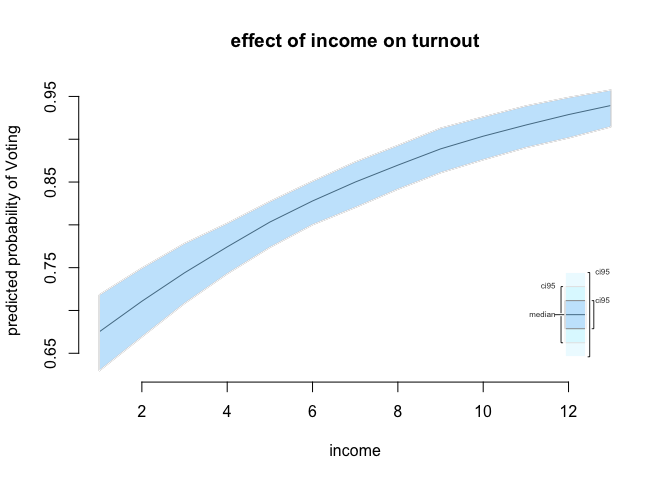
# plot income from lowest to highest
plot.ci (sim.income.seq,
ci = 95,
xlab = "income",
ylab = "predicted probability of Voting",
main = "effect of income on turnout")
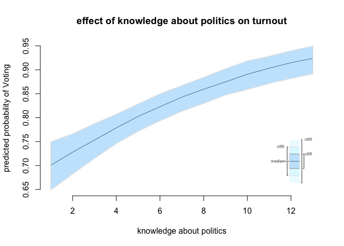
# plot polinfoindex from lowest to highest
plot.ci (sim.polinfoindex.seq,
         ci = 95,
         xlab = "knowledge about politics",
         ylab = "predicted probability of Voting",
         main = "effect of knowledge about politics on turnout")
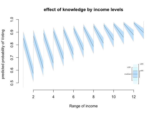
# plot resource variables from lowest to highest
plot.ci (sim.resource.seq,
         ci = 95,
         ylab = "predicted probability of Voting",
         main = "effect of knowledge by income levels")
The first plot illustrates the effect of income on turnout keeping all other variables in the model at their appropriate measures of central tendency. We predict income to increase turnout from roughly 67% at the lowest income level to roughly 93% at the highest income level.
Political knowledge, we predict, increases turnout from roughly 70% at the lowest knowledge level to roughly 92% at the highest knowledge level.
One thing to keep in mind here, the effect of varying income is done while keeping knowledge at the mean (and the other variables at means or modes as well). So, in our last plot we show the effect that political knowledge has at different income levels. At very low income levels increasing knowledge has a much larger effect than at very high levels of income. We may want to keep in mind though that both variables correlate. The extreme combinations, very high income and low knowledge and vice-versa may be uncommon.
cor.test(bes$income, bes$polinfoindex, mu = 0, use = "complete.obs")
    Pearson's product-moment correlation

data:  bes$income and bes$polinfoindex
t = 12.645, df = 4159, p-value < 2.2e-16
alternative hypothesis: true correlation is not equal to 0
95 percent confidence interval:
 0.1629757 0.2214996
sample estimates:
      cor
0.1924087
Our final theory is the sociological theory. We proceed by illustrating the effect of civic duty for an otherwise average voter.
# varying civic duty all else at appropriate measure of central tendency
x.civicduty.seq <- setx(z.full, civicduty = seq(min(bes$civicduty), max(bes$civicduty), 0.01),
                        polinfoindex = mean(bes$polinfoindex), income = mean(bes$income),
                        influence = mean(bes$influence),  partyid = 1, male = 0,
                        age = mean(bes$age), edu15 = 1, edu17 = 0, edu18 = 0,
                        edu19plus = 0, in_school = 0, in_uni = 0)


# simulation for civic duty
sim.civicduty <- sim(z.full, x.civicduty.seq)

# plot effect of civic duty
plot.ci (sim.civicduty,
         ci = 95,
         ylab = "predicted probability of Voting",
         main = "effect of civic duty on turnout")
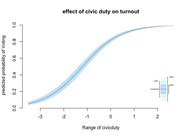
As we can see the effect of civic duty is extremely large. Remember, all other variables are held at their means or modes. So, we are talking about a voter who is average other than her sense of duty. At extremely low values of civic duty, voters are very unlikely to turnout while at very large values they are very likely to turnout. Uncertainty levels are very small. The effect of civicduty dwarfs the other effects. Overall, the sociological theory receives overwhelming support in terms of uncertainty (very small) and substantial effect (very large).