- Introduction
- 1. Introduction to Quantitative Analysis
- 2. Descriptive Statistics
- 3. T-test for Difference in Means and Hypothesis Testing
- 4. Bivariate linear regression models
- 5. Multiple linear regression models
- 6. Assumptions and Violations of Assumptions
- 7. Interactions
- 8. Panel Data, Time-Series Cross-Section Models
- 9. Binary models: Logit
- 10. Frequently Asked Questions
- 11. Optional Material
- 12. Datasets
- 13. R Resources
- 14. References
- Published with GitBook
2. Descriptive Statistics
2.2 Solutions
Exercise 1
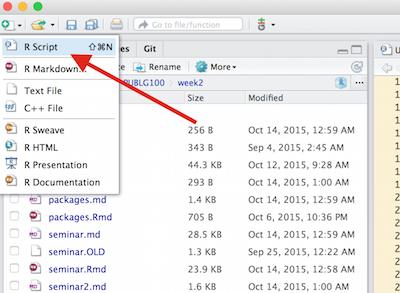
Create a new file called "assignment2.R" in your PUBLG100 folder and write all the solutions in it.
Solution
Exercise 2
Clear the workspace and set the working directory to your PUBLG100 folder.
Solution
Set the working directory with setwd() as we did in the seminar to where your course files are kept and verify it wih getwd(). Next, make sure to clear the workspace with the rm() function.
# Change your working directory
setwd("N:/PUBLG100")

# Check your working directory
getwd()

# clear the environment
rm(list = ls())
Exercise 3
Load the High School and Beyond dataset. Remember to load any necessary packages.
Solution
- Load the
readxlpackage using thelibrary()function. - Load the "hsb2.xlsx" dataset with the
read_excel()function. It is the same dataset that we worked with in the seminar. If it's not in your working directory then download it from the link provided in the exercise.
library(readxl)
student_data <- read_excel("hsb2.xlsx")
Exercise 4
Calculate the final score for each student by averaging the read, write, math, science, and socst scores and save it in a column called final_score.
Solution
We can use the apply() function to calculate the average just like we did in the seminar.
student_data$final_score <- apply(student_data[c("read", "write", "math", "science", "socst")],
                                  1,
                                  mean)

head(student_data)
   id female race ses schtyp prog read write math science socst
1  70      0    4   1      1    1   57    52   41      47    57
2 121      1    4   2      1    3   68    59   53      63    61
3  86      0    4   3      1    1   44    33   54      58    31
4 141      0    4   3      1    3   63    44   47      53    56
5 172      0    4   2      1    2   47    52   57      53    61
6 113      0    4   2      1    2   44    52   51      63    61
  final_score
1        50.8
2        60.8
3        44.0
4        52.6
5        54.0
6        54.2
Exercise 5
Calculate the mean, median and mode for the final_score.
Solution
Mean and median can be calculated with mean() and median() functions.
mean_final <- mean(student_data$final_score)
mean_final
[1] 52.384
median_final <- median(student_data$final_score)
median_final
[1] 53
Mode requires using the table() function and sorting the result with sort().
mode_final <- sort(table(student_data$final_score), decreasing = TRUE)[1]
mode_final
50.6
   5
Exercise 6
Create a factor variable called school_type from schtyp using the following codes:
- 1 = Public schools
- 2 = Private schools
Solution
Use the factor() function and pass it c("Public", "Private") as factor labels.
student_data$school_type <- factor(student_data$schtyp, labels = c("Public", "Private"))
Exercise 7
How many students are from private schools and how many are from public schools?
Solution
Get the frequency table with the table() function.
table(student_data$school_type)
 Public Private
    168      32
Exercise 8
Calculate the variance and standard deviation for final_score from each school type.
Solution
- Subset the data for private and schools using
subset()function andschool_type == "Public". - Use
var()to calculate the variance. - Use
sd()to calculate the standard deviation.
public_school <- subset(student_data, school_type == "Public")
public_var <- var(public_school$final_score)
public_sd <- sd(public_school$final_score)
Variance for public schools is 70.9795495, while standard deviation is 8.4249362.
Now repeat the same steps for private schools.
private_school <- subset(student_data, school_type == "Private")
private_var <- var(private_school$final_score)
private_sd <- sd(private_school$final_score)
Variance for private schools is 41.1064516, while standard deviation is 6.4114313.
Exercise 9
Find out the ID of the students with the highest and lowest final_score from each school type.
Solution
- Use
which.min()andwhich.max()to find out the row number of the student with the lowest and highest final scores from public schools. - Use the
idvariable to get the student ID.
top_public_student <- which.max(public_school$final_score)
top_public_student_id <- public_school[top_public_student,]$id

bottom_public_student <- which.min(public_school$final_score)
bottom_public_student_id <- public_school[bottom_public_student,]$id
- Student ID 132 has the highest final score of 68.6 from public schools.
- Student ID 45 has the lowest final score of 33 from public schools.
Next, repeat the same steps for private schools.
top_private_student <- which.max(private_school$final_score)
top_private_student_id <- private_school[top_private_student,]$id

bottom_private_student <- which.min(private_school$final_score)
bottom_private_student_id <- private_school[bottom_private_student,]$id
- Student ID 180 has the highest final score of 66.8 from private schools.
- Student ID 196 has the lowest final score of 43.2 from private schools.
Exercise 10
Find out the 20th, 40th, 60th and 80th percentiles of final_score.
Solution
Use the quartile() function and pass it c(0.2, 0.4, 0.6, 0.8) to get the 20th, 40th, 60th and 80th percentiles.
quantile(student_data$final_score, c(0.2, 0.4, 0.6, 0.8))
  20%   40%   60%   80%
44.56 50.44 54.68 59.48
Exercise 11
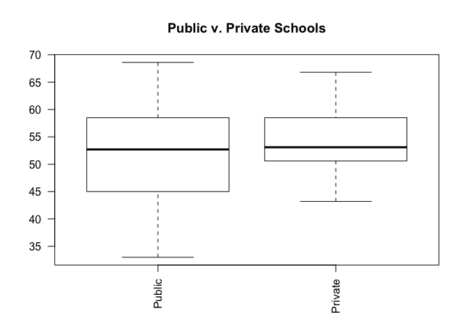
Create box plot for final_score and school_type factor variable to show the difference between final_score at public schools vs. private schools.
Solution
Use the plot() function to generate a box plot. Since the data we're passing is a factor variable, plot() automatically creates a box plot.
plot(student_data$school_type,
     student_data$final_score,
     main = "Public v. Private Schools",
     las = 2)