- Introduction
- 1. Introduction to Quantitative Analysis
- 2. Descriptive Statistics
- 3. T-test for Difference in Means and Hypothesis Testing
- 4. Bivariate linear regression models
- 5. Multiple linear regression models
- 6. Assumptions and Violations of Assumptions
- 7. Interactions
- 8. Panel Data, Time-Series Cross-Section Models
- 9. Binary models: Logit
- 10. Frequently Asked Questions
- 11. Optional Material
- 12. Datasets
- 13. R Resources
- 14. References
- Published with GitBook
9. Binary models: Logit
9.1 Seminar
Setting a Working Directory
Before you begin, make sure to set your working directory to a folder where your course related files such as R scripts and datasets are kept. We recommend that you create a PUBLG100 folder for all your work. Create this folder on N: drive if you're using a UCL computer or somewhere on your local disk if you're using a personal laptop.
Once the folder is created, use the setwd() function in R to set your working directory.
| Recommended Folder Location | R Function | |
|---|---|---|
| UCL Computers | N: Drive | setwd("N:/PUBLG100") |
| Personal Laptop (Windows) | C: Drive | setwd("C:/PUBLG100") |
| Personal Laptop (Mac) | Home Folder | setwd("~/PUBLG100") |
After you've set the working directory, verify it by calling the getwd() function.
getwd()
Now download the R script for this seminar from the "Download .R Script" button above, and save it to your PUBLG100 folder.
library(Zelig) # load BEFORE dplyr!!!
library(foreign) # to load .dta files
library(lmtest) # for likelihood ratio test
library(texreg) # regression tables
Warning: package 'texreg' was built under R version 3.2.3
library(dplyr) # data manipulation/ summary statistics

# clear environment
rm(list = ls())
Before you start, please make sure that you loaded the dplyr package last. Loading Zelig after dplyr may lead to problems.
Loading Data
We use a subset of the 2005 face-to-face British post election study to explain turnout. We drop missing values (missings are on the same observations for all variables). We also rename Gender to male because 1 stands for men.
Disclaimer: We use a slightly modified version of the data set. For your own research please visit the British Election Study website.
# load British post election study
bes <- read.dta("http://uclspp.github.io/PUBLG100/data/bes.dta")
head(bes)
  cs_id Turnout Vote2001 Income Age Gender PartyID Influence Attention
1     1       0        1      4  76      0       1         1         8
2     2       1        1      5  32      1       0         3         8
3     3       1       NA     NA  NA     NA      NA        NA        NA
4     4       0        1      1  35      0       0         1         1
5     5       1        1      7  56      1       0         1         9
6     6       1        1      4  76      0       1         4         8
  Telephone LeftrightSelf CivicDutyIndex polinfoindex edu15 edu16 edu17
1         1             7             20            7     1     0     0
2         1             6             15            5     0     1     0
3        NA            NA             NA           NA    NA    NA    NA
4         0             5             26            1     0     1     0
5         1             9             16            7     0     0     1
6         1             8             16            4     0     1     0
  edu18 edu19plus in_school in_uni CivicDutyScores
1     0         0         0      0      -0.6331136
2     0         0         0      0       1.4794579
3    NA        NA        NA     NA              NA
4     0         0         0      0      -2.1466281
5     0         0         0      0       1.0324940
6     0         0         0      0       0.3658024
# frequency table of voter turnout
table(bes$Turnout)
   0    1
1079 3712
# rename Gender to male b/c 1 = male & remove missings
bes <- bes %>%
  rename(male = Gender) %>%
  na.omit()
Dplyr summarise()
We will look at summary statistics by groups using group_by() and summarise(). First we group by the variable male and then we calculate mean and standard deviation of voter turnout. The syntax is: summarise(new.variable = summary.statistic). With summarise_each() you can calculate descriptive statistics for multiple columns.
# mean and standard deviation for Turnout by gender
bes %>%
  group_by(male) %>%
  summarise(avg_turnout = mean(Turnout), sd_turnout = sd(Turnout))
Source: local data frame [2 x 3]

   male avg_turnout sd_turnout
  (dbl)       (dbl)      (dbl)
1     0   0.7465517  0.4350791
2     1   0.7332971  0.4423559
# mean for multiple columns using "summarise_each"
bes %>%
  group_by(male) %>%
  summarise_each(funs(mean), Turnout, Vote2001, Age, LeftrightSelf,
                 CivicDutyIndex, polinfoindex)
Source: local data frame [2 x 7]

   male   Turnout  Vote2001      Age LeftrightSelf CivicDutyIndex
  (dbl)     (dbl)     (dbl)    (dbl)         (dbl)          (dbl)
1     0 0.7465517 0.8400862 51.04914      5.397414       17.35216
2     1 0.7332971 0.8365019 50.75394      5.409560       17.76697
Variables not shown: polinfoindex (dbl)
Regression with a binary dependent variable
We use the glm() function to estimate a logistic regression. The syntax is familiar from lm() and plm(). "glm" stands for generalized linear models and can be used to estimate many different models. The argument family = binomial(link = "logit") tells glm that we have a binary dependent variable that our link function is the cumulative logistic function.
# logit model
model1 <- glm(Turnout ~ Income + polinfoindex + male + edu15 + edu17 + edu18 +
                edu19plus + in_school + in_uni, family = binomial(link = "logit"),
              data = bes)

# regression output
screenreg(model1)
============================
                Model 1
----------------------------
(Intercept)        -1.14 ***
                   (0.15)
Income              0.03
                   (0.02)
polinfoindex        0.38 ***
                   (0.02)
male               -0.35 ***
                   (0.08)
edu15               0.38 ***
                   (0.10)
edu17               0.46 **
                   (0.15)
edu18               0.11
                   (0.14)
edu19plus           0.24 *
                   (0.12)
in_school           0.15
                   (0.39)
in_uni             -0.72 **
                   (0.25)
----------------------------
AIC              4401.20
BIC              4464.53
Log Likelihood  -2190.60
Deviance         4381.20
Num. obs.        4161
============================
*** p < 0.001, ** p < 0.01, * p < 0.05
Predicted Probabilities and Predictive Power
To assess the predictive power of our model we will check the percentage of cases that it correctly predicts. If we look at the mean of Turnout we will see that is 0.74. That means 74% of the respondents said that they turned out to vote. If you predict for every respondent that they voted, you will be right for 74% of the people. That is the naive guess and the benchmark for our model. If we predict more than 74% of cases correctly our model adds value.
Below we will estimate predicted probabilities for each observation. That is, the probability our model assigns that a respondent will turn out to vote for every person in our data. To do so we use the predict() function. Type help(predict.glm) for information on all arguments. We use: predict(model.name, type = "response"). The first argument is the glm object (our model name) and the second specifies that we want predicted probabilities.
# predicted probabilities for all respondents
predicted.probabilities <- predict(model1, type = "response")
Now that we have assigned probabilities to people turning out, we have to translate those into outcomes. Turnout is binary. A straightforward way, would be to say: We predict that all people with a predicted probability above 50% vote and all with predicted probabilities below or equal to 50% abstain. We specify this threshold below.
# threshold to translate predicted probabilities into outcomes
threshold <- .5
We create a new variable expected.values that is 1 if our predicted probability (predicted.probabilites) is larger than 0.5 and 0 otherwise. This is easily done with the ifelse() function. The syntax is as follows:
ifelse( condition, what to do if condition is true, what to do if condition is false)
# set prediction to 1 if predicted probability is larger than 0.5 and put 0 otherwise
expected.values <- ifelse(predicted.probabilities > threshold, yes = 1, no = 0)
All we have to do now is to compare our expected values of turnout against the actually observed values of turnout. This will produce a table like this:
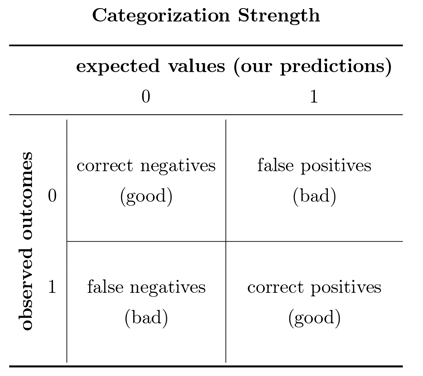
The threshold that we set is directly related to the proportion of type I to type II errors. Increasing the threshold will reduce the number of false positives but increase the number of false negatives and vice versa. The default choice is a threshold of 0.5. However, you may imagine situations where on type of error is more costly than the other. For example, given the cost of civil wars, a model predicting civil war may focus on reducing false negatives at the cost of a larger fraction of false positives.
We proceed by producing a table of predictions against actual outcomes. With that we will calculate the percentage of correctly predicted cases and compare that to the naive guess. We have the actually observed cases in our dependent variable (Turnout). The table is just a frequency table. The percentage of correctly predicted cases is simply the sum of correctly predicted cases over the number of cases.
 # actually observed outcomes
observed <- bes$Turnout

# putting observed outcomes and predicted outcomes into a table
outcome.table <- table(observed,expected.values)
outcome.table
        expected.values
observed    0    1
       0  160  919
       1  108 2974
# correctly predicted cases:
# (correct negatives + correct positives) / total number of outcomes
correctly.predicted <- (outcome.table[1,1] + outcome.table[2,2]) / sum(outcome.table)
correctly.predicted
[1] 0.7531843
# comparing rate of correctly predicted to naive guess
mean(bes$Turnout)
[1] 0.7406873
You can see that our model outperforms the naive guess slightly. The more lopsided the distribution of your binary dependent variable, the harder it is to build a successful model.
Joint hypothesis testing
We add more explanatory variables to our model: Influence and Age. Influence corresponds to a theory we want to test while Age is a socio-economic control variable.
We want to test two theories: the rational voter model and the resource theory.
Influence operationalises a part of the rational voter theory. In that theory citizens are more likely to turnout the more they belive that their vote matters. The variable Influence measures the subjective feeling of being able to influence politics.
The variables Income and polinfoindex correspond to a second theory which states that people who have more cognitive and material resources are more likely to participate in politics.
Depending on whether the coefficients corresponding to the respective theories are significant or not, we can say something about whether these theories help to explain turnout.
The remaining variables for gender, education and the added variable Age are socio-economic controls. We added age because previous research has shown that political participation changes with the life cycle.
# esimate the new model 2 including Influence and Age
model2 <- glm(Turnout ~ Income + polinfoindex + Influence + male + Age +
                edu15 + edu17 + edu18 + edu19plus + in_school + in_uni,
              family = binomial(link = "logit"), data = bes)

# regression table comparing model 1 and model 2
screenreg( list(model1, model2) )
==========================================
                Model 1       Model 2
------------------------------------------
(Intercept)        -1.14 ***     -3.90 ***
                   (0.15)        (0.22)
Income              0.03          0.15 ***
                   (0.02)        (0.02)
polinfoindex        0.38 ***      0.25 ***
                   (0.02)        (0.02)
male               -0.35 ***     -0.36 ***
                   (0.08)        (0.08)
edu15               0.38 ***     -0.34 **
                   (0.10)        (0.11)
edu17               0.46 **       0.36 *
                   (0.15)        (0.16)
edu18               0.11          0.14
                   (0.14)        (0.15)
edu19plus           0.24 *        0.01
                   (0.12)        (0.13)
in_school           0.15          1.13 **
                   (0.39)        (0.40)
in_uni             -0.72 **      -0.05
                   (0.25)        (0.27)
Influence                         0.21 ***
                                 (0.02)
Age                               0.05 ***
                                 (0.00)
------------------------------------------
AIC              4401.20       4003.90
BIC              4464.53       4079.90
Log Likelihood  -2190.60      -1989.95
Deviance         4381.20       3979.90
Num. obs.        4161          4161
==========================================
*** p < 0.001, ** p < 0.01, * p < 0.05
The variables corresponding to the resource theory are Income and polinfoindex. In our model 2 (the one we interpret), both more income and more interest in politics are related to a higher probability to turn out to vote. That is in line with the theory. Interestingly, income was previously insignificant in model 1. It is quite likely that model 1 suffered from omitted variable bias. Age, e.g., may be related to income and turnout.
As the rational voter model predicts, a higher subjective probability to cast a decisive vote, which we crudly proxy by the feeling to be able to influence politics, does correspond to a higher probability to vote as indicated by the positive significant effect of our Influence variable.
We will test if model 2 does better at predicting turnout than model 1. We use the likelihood ratio test. This is warranted because we added two variables and corresponds to the F-test in the OLS models estimated before. You can see values for the logged likelihood in the regression table. You cannot in general say whether a value for the likelihood is small or large but you can use it to compare models that are based on the same sample. A larger log-likelihood is better. Looking at the regression table we see that the log-likelihood is larger in model 2 than in model 1. We use the lmtest package to test whether that difference is statistically significant using the lrtest() function. The syntax is the following:
lrtest(model with less variables, model with more variables)
# the likelihood ratio test
lrtest(model1, model2)
Likelihood ratio test

Model 1: Turnout ~ Income + polinfoindex + male + edu15 + edu17 + edu18 +
    edu19plus + in_school + in_uni
Model 2: Turnout ~ Income + polinfoindex + Influence + male + Age + edu15 +
    edu17 + edu18 + edu19plus + in_school + in_uni
  #Df  LogLik Df Chisq Pr(>Chisq)
1  10 -2190.6
2  12 -1990.0  2 401.3  < 2.2e-16 ***
---
Signif. codes:  0 '***' 0.001 '**' 0.01 '*' 0.05 '.' 0.1 ' ' 1
# Akaike's Information Criterion
AIC(model1, model2)
       df      AIC
model1 10 4401.200
model2 12 4003.901
# Bayesian Infromation Criterion
BIC(model1, model2)
       df      BIC
model1 10 4464.535
model2 12 4079.903
The p-value in the likelihood ratio test is smaller than 0.05. Therefore, the difference between the two log-likelihoods is statistically significant which means that model 2 is better at explaining turnout.
AIC and BIC agree, model 2 has better fit.
Substantial interpretation
Due to the functional form of the cumulative logistic function, the effect of a change in an independent variable depends on the level of the independent variable, i.e. they are not constant. Interpretation is nonetheless easily accomplished using Zelig. We pick meaningful scenarios and predict the probability that a person will vote based on the scenarios. First, we re-estimate model 2 using zelig.
# re-estimate model 2 using Zelig
z.m2 <- zelig(Turnout ~ Income + polinfoindex + Influence + male + Age + edu15 +
                edu17 + edu18 + edu19plus + in_school + in_uni, model = "logit",
              data = bes, cite = FALSE)
What are meaningful scenarios? A meaningful scenario is a set of covariate values that corresponds to some case that is interesting in reality. For example, you may want to compare a women with 18 years of education to a man with 18 years of education while keeping all other variables at their means, medians or modes.
We set binary variables to their modes, ordinally scaled variables to their medians and interval scaled variables to their means. By doing so for all variables except education and gender, we compare the average women with 18 years of education to the average man with 18 years of education.
# average man with 18 years of education
x.male.18edu <- setx(z.m2, male = 1, edu18 = 1, Income = mean(bes$Income),
                     polinfoindex = mean(bes$polinfoindex), Influence = mean(bes$Influence),
                     Age = mean(bes$Age), edu15 = 0, edu17 = 0,  edu19plus = 0,
                     in_school = 0, in_uni = 0)

# check covariate values (if you have missings here, the simulation will not work)
t(x.male.18edu$values)
     male edu18 Income   polinfoindex Influence Age      edu15 edu17
[1,] 1    1     5.321557 5.409277     3.608508  50.91853 0     0
     edu19plus in_school in_uni
[1,] 0         0         0
# average woman with 18 years of education
x.female.18edu <- setx(z.m2, male = 0, edu18 = 1, Income = mean(bes$Income),
                       polinfoindex = mean(bes$polinfoindex), Influence = mean(bes$Influence),
                       Age = mean(bes$Age), edu15 = 0, edu17 = 0,  edu19plus = 0,
                       in_school = 0, in_uni = 0)

# check covariate values (if you have missings here, the simulation will not work)
t(x.female.18edu$values)
     male edu18 Income   polinfoindex Influence Age      edu15 edu17
[1,] 0    1     5.321557 5.409277     3.608508  50.91853 0     0
     edu19plus in_school in_uni
[1,] 0         0         0
Note: Do not worry about the t() around the covariate vectors. This simply transposes the vector so that it is printed horizontally instead of vertically.
You see that the only difference between the covariate values in the two scenarios is gender. Therefore, we can compare a women and a man that are identical in all other attributes in our model. This is what keeping other variables constant means.
Now all we have to do is simulate and compare the results.
# make simulation replicable, the values in set.seed() do not matter
set.seed(123)

# simulate with our two scenarios
s.out <- sim(z.m2, x = x.female.18edu, x1 = x.male.18edu)

# outcomes, check especially first differences
summary(s.out)
Model:  logit
Number of simulations:  1000

Values of X
  (Intercept)   Income polinfoindex Influence male      Age edu15 edu17
1           1 5.321557     5.409277  3.608508    0 50.91853     0     0
  edu18 edu19plus in_school in_uni
1     1         0         0      0
attr(,"assign")
 [1]  0  1  2  3  4  5  6  7  8  9 10 11

Values of X1
  (Intercept)   Income polinfoindex Influence male      Age edu15 edu17
1           1 5.321557     5.409277  3.608508    1 50.91853     0     0
  edu18 edu19plus in_school in_uni
1     1         0         0      0
attr(,"assign")
 [1]  0  1  2  3  4  5  6  7  8  9 10 11

Expected Values: E(Y|X)
  mean    sd   50%  2.5% 97.5%
 0.838 0.019 0.838 0.795 0.873

Expected Values: E(Y|X1)
  mean    sd   50% 2.5% 97.5%
 0.783 0.025 0.784 0.73 0.832

Predicted Values: Y|X
     0     1
 0.162 0.838

Predicted Values: Y|X1
     0     1
 0.217 0.783

First Differences: E(Y|X1) - E(Y|X)
   mean    sd    50%   2.5%  97.5%
 -0.054 0.014 -0.054 -0.082 -0.028
For the average woman (in our sample) with 18 years of education, we predict a probability of 84% that she will vote. Our uncertainty is plus and minus 4% on the 95% confidence level. For her male counterpart, we predict the probability of turnout to be 78% (plus and minus 5% based on the 95% confidence interval). Is the difference between them statistically significant or put differently is our hypothetical woman more likely to vote than our hypothetical man?
To check we look at the first difference. The difference is 6 percentage points on average and between 8 percentage points and 3 percentage points based on the 95% confidence interval.
Note: We had to look at the first difference to see if our hypothetical subjects are statistically different with respect to the predicted probability of voting. If you were to look at the confidence intervals of the expected values only, you would see an overlap.
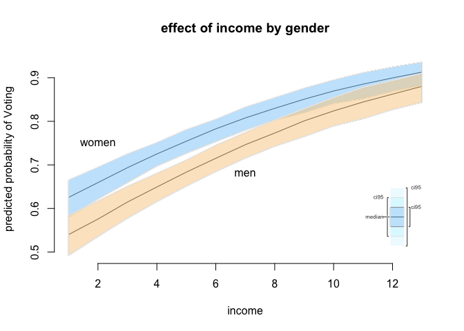
Our next step will be to compare two groups like men and women while varying another continuous variable from lowest to highest. We use income here. So, we set a sequence for income, vary gender and keep every other variable constant at its appropriate measure of central tendency.
# women with income levels from lowest to highest (notice we put education to the mode)
x.fem <- setx(z.m2, male = 0, Income = 1:13, polinfoindex = mean(bes$polinfoindex),
              Influence = mean(bes$Influence), Age = mean(bes$Age),
              edu15 = 1, edu17 = 0, edu18 = 0, edu19plus = 0, in_school = 0, in_uni = 0)

# men with income levels from lowest to highest (notice we put education to the mode)
x.mal <- setx(z.m2, male = 1, Income = 1:13, polinfoindex = mean(bes$polinfoindex),
              Influence = mean(bes$Influence), Age = mean(bes$Age),
              edu15 = 1, edu17 = 0, edu18 = 0, edu19plus = 0, in_school = 0, in_uni = 0)
If you want to check the values we have set again this would work slightly different this time because we have set Income to a sequence. You will see the values that you have set if you type names(x.fem) and names(x.mal).
# simulation
s.out2 <- sim(z.m2, x = x.fem, x1 = x.mal)
We will illustrate our results. The plot function here is slightly different as well. You use plot.ci() instead of the usual plot() function.
# final plot
plot.ci (s.out2,
         ci = 95,
         xlab = "income",
         ylab = "predicted probability of Voting",
         main = "effect of income by gender")

# add labels manually
text( x = 2, y = .75, labels = "women" )
text( x = 7, y = .68, labels = "men" )
Exercises
| Theory | Mechanism | Corresponding Variables |
|---|---|---|
| Resource Theory | More resources reduce transaction costs for political participation. People who possess more knowledge about the political system and who are wealthier will be more likely to vote. | Income and polinfoindex |
| Rational Voter | Voters are motivated by three variables. Costs of voting, benefits of voting and the probability of casting the decisive vote. The first decreases the probability of voting, the latter two increase the probability of voting. | Influence as the probability of casting the decisive vote. |
| Sociological Theory | People with more social capital are well integrated in civil society and feel a greater sense of duty to contribute to society while at the same time having a sense that they can shape society. | CivicDutyScores |
- Estimate a model similar to model 2 in the seminar and add Civic Duty (
CivicDutyScores) and party identification (PartyID). Show and discuss descriptive statistics of the variables in a meaningful way. E.g.: what does a unit change in a variable mean, are variables comparable. Do this for all variables but concentrate your discussion on the interesting ones. - Do joint hypothesis testing and explain your results. You have added two variables, so the comparison should be to the model without those two new variables.
- What is the model's predictive power? How well does it do compared to the naive guess and model 2, that we estimated in class?
- How many false positives and how many false negatives to we get in our full final model?
- What is the trade-off between the errors we make when increasing the cut-off point to 0.7?
- Choose an average voter who does not identify with a party and show how likely that voter is to vote. Compare that to a voter who identifies with a political party. Interpret your results.
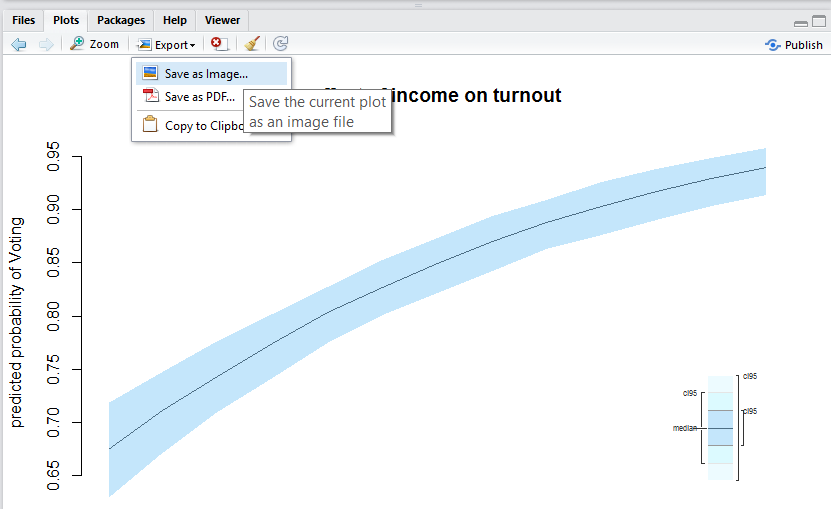
- Thoroughly interpret the full final model in the light of all three theories in substantial terms. Use at least one plot to illustrate your results. Export that plot as a "png" or "pdf" file and put it in word document. If you cannot do this, seek help in the office hours!
You will need this in the exam!!
Saving an R plot is easy. In the plot window, you click on export and then you just choose the file format you want ("png" or "pdf" will work best).