- Introduction
- 1. Introduction to Quantitative Analysis
- 2. Descriptive Statistics
- 3. T-test for Difference in Means and Hypothesis Testing
- 4. Bivariate linear regression models
- 5. Multiple linear regression models
- 6. Assumptions and Violations of Assumptions
- 7. Interactions
- 8. Panel Data, Time-Series Cross-Section Models
- 9. Binary models: Logit
- 10. Frequently Asked Questions
- 11. Optional Material
- 12. Datasets
- 13. R Resources
- 14. References
- Published with GitBook
3. T-test for Difference in Means and Hypothesis Testing
3.1 Seminar
Setting a Working Directory
Before you begin, make sure to set your working directory to a folder where your course related files such as R scripts and datasets are kept. We recommend that you create a PUBLG100 folder for all your work. Create this folder on N: drive if you're using a UCL computer or somewhere on your local disk if you're using a personal laptop.
Once the folder is created, use the setwd() function in R to set your working directory.
| Recommended Folder Location | R Function | |
|---|---|---|
| UCL Computers | N: Drive | setwd("N:/PUBLG100") |
| Personal Laptop (Windows) | C: Drive | setwd("C:/PUBLG100") |
| Personal Laptop (Mac) | Home Folder | setwd("~/PUBLG100") |
After you've set the working directory, verify it by calling the getwd() function.
getwd()
Now download the R script for this seminar from the "Download .R Script" button above, and save it to your PUBLG100 folder.
rm(list=ls()) # clear workspace
Loading Dataset in Stata Format
In the last two seminars we worked with data sets in CSV and Excel (.xlsx) formats and learned how to use the readxl package. In this seminar, we will be loading data from Stata file formats. One of the core packages that comes pre-installed with R allows us to directly read a file saved in Stata format. The package is called foreign and it's designed to provide support for non-native (or "foreign") file formats.
The function we need to use for loading a file in Stata format is read.dta(). We use data from the Institute for Quality of Governance today. You can download a codebook for the variables here. So, let's load the data set and do our usual routine of getting to know our data.
library(foreign) # to work with foreign file formats

# loading a STATA format data set (remember to load the library foreign 1st)
world.data <- read.dta("http://uclspp.github.io/PUBLG100/data/QoG2012.dta")

# the dimensions: rows (observations) and columns (variables)
dim(world.data)
[1] 194 7
# the variable names
names(world.data)
[1] "h_j"         "wdi_gdpc"    "undp_hdi"    "wbgi_cce"    "wbgi_pse"
[6] "former_col"  "lp_lat_abst"
# the top ten rows and all columns
world.data[ 1:10 , ]
   h_j   wdi_gdpc undp_hdi   wbgi_cce   wbgi_pse former_col lp_lat_abst
1   -5   628.4074       NA -1.5453584 -1.9343837          0   0.3666667
2   -5  4954.1982    0.781 -0.8538115 -0.6026081          0   0.4555556
3   -5  6349.7207    0.704 -0.7301510 -1.7336243          1   0.3111111
4   NA         NA       NA  1.3267342  1.1980436          0   0.4700000
5   -5  2856.7517    0.381 -1.2065741 -1.4150945          1   0.1366667
6   NA 13981.9795    0.800  0.8624368  0.7084046          1   0.1892222
7   -5  2980.8616    0.746 -0.9852442 -1.1296966          0   0.4477778
8   -5  8584.8857    0.853 -0.7264611 -1.0361214          1   0.3777778
9    1 32201.2227    0.946  1.8478516  1.2044924          0   0.3000000
10   1 32082.7168    0.934  1.9580450  1.3096740          0   0.5244445
Dplyr Package
Today we introduce another package called dplyr. It is a package that makes it easier for you to work with data sets. It includes functions that let you rename variables, pick out observations that fulfill certain conditions, like gender==female, lets you select certain variables and many more things. From now on, we will introduce a new function of dplyr every week. But first we will install the package with install.packages("dplyr"). Each time you want to use the package you have to load it with library(dplyr).
install.packages("dplyr")
Installing package into '/Users/altaf/Library/R/3.2/library'
(as 'lib' is unspecified)


The downloaded binary packages are in
    /var/folders/62/x92vvd_n08qb3vw5wb_706h80000gp/T//Rtmpj8Oitn/downloaded_packages
Dplyr: rename()
The first function from the dplyr package that will make your live easier is rename(). You may have noticed that the variable names in our data are quite cryptic. With the help of the codebook we understand what is going on but we may want to use more intuitive variable names instead. The rename() function lets you do that. Remember, to use rename(), the dplyr package must be loaded with library(dplyr). We want to rename the variable h_j which is an indicator variable, where 1 means that an independent judiciary exists and the other category means that the executive branch has some control over the judiciary.
Here's a list of arguments we need to provide to the rename() function and their descriptions.
rename(dataset, expression)
| Argument | Description |
|---|---|
| dataset | The first argument is the name of your data set (we have called it world.data). |
| expression | The second argument is the expression that assigns a new variable name to an existing variable in our dataset. For example: new.variable = existing.variable. |
In order to save your new variable name in the data set world.data, we have to assign our renamed variable to the data set using the <- symbol. We will now rename h_j into indep.judi
# load dplyr
library(dplyr)
# dataset.name <- rename(argument1, argument2 = argument3)
# h_j = 1 means there is an independent judiciary
# rename h_j to indep.judi

# rename a variable and save the result in our data frame
world.data <- rename( world.data, indep.judi = h_j )

# check the result
names(world.data)
[1] "indep.judi"  "wdi_gdpc"    "undp_hdi"    "wbgi_cce"    "wbgi_pse"
[6] "former_col"  "lp_lat_abst"
T-test
We are interested in whether there is a difference in income between countries that have an independent judiciary and countries that do not have an independent judiciary. The t-test is the appropriate test statistic for an interval level dependent variable and a binary independent variable. Our interval level dependent variable is wdi_gdpc which is GDP per capita taken from the World Development Indicators of the World Bank. Our binary independent variable is indep.judi. We take a look at our independent variable first.
# frequency table of binary independent variable
table(world.data$indep.judi)
 -5   1
105  64
As we can see the categories are numbered 1 and -5. We are used to 0 and 1. The codebook tells us that 1 means that the country has an independent judiciary. We will now turn indep.judi into a factor variable like we did last time using the factor() function.
# creating a factor variable
world.data$indep.judi <- factor(world.data$indep.judi,
                                labels = c("contr. judiciary", "indep. judiciary"))

# checking the result
world.data[ 1:10, ]
         indep.judi   wdi_gdpc undp_hdi   wbgi_cce   wbgi_pse former_col
1  contr. judiciary   628.4074       NA -1.5453584 -1.9343837          0
2  contr. judiciary  4954.1982    0.781 -0.8538115 -0.6026081          0
3  contr. judiciary  6349.7207    0.704 -0.7301510 -1.7336243          1
4              <NA>         NA       NA  1.3267342  1.1980436          0
5  contr. judiciary  2856.7517    0.381 -1.2065741 -1.4150945          1
6              <NA> 13981.9795    0.800  0.8624368  0.7084046          1
7  contr. judiciary  2980.8616    0.746 -0.9852442 -1.1296966          0
8  contr. judiciary  8584.8857    0.853 -0.7264611 -1.0361214          1
9  indep. judiciary 32201.2227    0.946  1.8478516  1.2044924          0
10 indep. judiciary 32082.7168    0.934  1.9580450  1.3096740          0
   lp_lat_abst
1    0.3666667
2    0.4555556
3    0.3111111
4    0.4700000
5    0.1366667
6    0.1892222
7    0.4477778
8    0.3777778
9    0.3000000
10   0.5244445
# a frequency table of indep.judi
table(world.data$indep.judi)
contr. judiciary indep. judiciary
             105               64
Now, we check the summary statistics of our dependent variable GDP per captia.
summary(world.data$wdi_gdpc)
   Min. 1st Qu.  Median    Mean 3rd Qu.    Max.    NA's
  226.2  1768.0  5326.0 10180.0 12980.0 63690.0      16
To get a first idea of whether our intuition, countries with an independent judiciary are richer, is true, we create sub samples of the data by judiciary and then check the mean GDP per capita. You may have noticed that wdi_gdpc contains 16 missing values called NA's by the summary() function. In order to calculate the mean we have to tell the mean() function what to do with them. The argument na.rm = TRUE removes all missings. Therefore, whenever you take the mean of a variable containing missing values you type: mean(variable.name, na.rm = TRUE).
# creating subsets of our data by the status of the judiciary
free.legal <- subset(world.data, indep.judi == "indep. judiciary")
contr.legal <- subset(world.data, indep.judi == "contr. judiciary")

# mean income levels, we remove missings
mean(free.legal$wdi_gdpc, na.rm = TRUE)
[1] 17826.59
mean(contr.legal$wdi_gdpc, na.rm = TRUE)
[1] 5884.882
Finally, we use the t.test() function. The syntax of a t.test for a binary dependent variable and an interval independent variable is:
t.test(formula, mu, alt, conf)
Lets have a look at the arguments.
| Arguments | Description |
|---|---|
formula |
The formula describes the relationship between the dependent and independent variables, for example dependent.variable ~ independent.variable |
mu |
Here, we set the null hypothesis. Suppose, there was no difference in income between countries that have an independent judiciary and those which do not. We would then expect that if we take the mean of income in both groups they should not differ too much from one another and the difference in means should not be significantly different from 0. So, when someone claims countries with an independent judiciary are richer, we would test this claim against the null hypothesis that there is no difference. Thus, we set mu = 0. |
alt |
There are two alternatives to the null hypothesis that the difference in means is zero. The difference could either be smaller or it could be larger than zero. To test against both alternatives, we set alt = "two.sided". |
conf |
Here, we set the level of confidence that we want in rejecting the null hypothesis. Common confidence intervals are: 90%, 95% and 99%. |
Lets run the test.
# t.test
# Interval DV (GDP per captia)
# Binary IV (independent judiciary)
t.test(world.data$wdi_gdpc ~ world.data$indep.judi, mu=0, alt="two.sided", conf=0.95)
    Welch Two Sample t-test

data:  world.data$wdi_gdpc by world.data$indep.judi
t = -6.0094, df = 98.261, p-value = 3.165e-08
alternative hypothesis: true difference in means is not equal to 0
95 percent confidence interval:
 -15885.06  -7998.36
sample estimates:
mean in group contr. judiciary mean in group indep. judiciary
                      5884.882                      17826.591
Lets interpret the results you get from t.test(). The first line is data: dependent variable by independent variable. This tells you that you are trying to find out whether there is a difference in means of your dependent variable by the groups of an independent variable. In our example: Do countries with independent judiciaries have different mean income levels than countries without independent judiciaries? In the following line you see the t-value, the degrees of freedom and the p-value. Knowing the t-value and the degrees of freedom you can check in a table on t distributions how likely you were to observe this data, if the null-hypothesis was true. The p-value gives you this probability directly. A p-value of 0.02 means that the probability to see this data given that there is no difference in incomes between countries with and without independent judiciaries, is 2%. In the next line you see the 95% confidence interval because we specified conf=0.95. If you were to take 100 samples and in each you checked the means of the two groups, 95 times the difference in means would be within the interval you see there. At the very bottom you see the means of the dependent variable by the two groups of the independent variable. These are the means that we estimated above. In our example, you see the mean income levels in countries were the executive has some control over the judiciary, and in countries were the judiciary is independent.
Pearson's r
When we want to test for a correlation between two variables that are at least interval scaled, we use Pearson's r. We want to test the relationship between control of corruption wbgi_cce and the human development index undp_hdi. Specifically, the human development index is our dependent variable and control of corruption is our independent variable. We will quickly rename the variables like we have learned above.
# renaming variables
world.data <- rename(world.data, hdi = undp_hdi)
world.data <- rename(world.data, cont.corr = wbgi_cce)
A good way to get an idea about a possible relationship between two interval scaled variables is to do a scatter plot like we have done last week.
# scatterplot
plot( x = world.data$cont.corr,
      y = world.data$hdi,
      xlim = c(xmin = -2, xmax = 3),
      ylim = c(ymin = 0, ymax = 1),
      frame = FALSE,
      xlab = "World Bank Control of Corruption Index",
      ylab = "UN Development Programme Human Development Index",
      main = "Relationship b/w Quality of Institutions and Quality of Life")
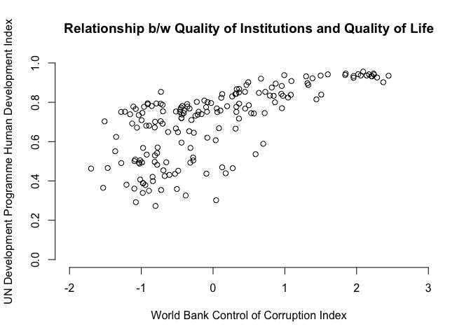
You can probably spot that there is likely a positive relationship between control of corruption and the human development index. To see the slope, or in other words, the correlation exactly and whether that correlation is significantly different from zero we estimate Pearson's r with the cor.test() function. This will give us the mean correlation as well as an a confidence interval around the mean. The cor.test() function expects the following arguments:
cor.test(x, y, use, conf.level)
These arguments have the following meanings:
| Argument | Description |
|---|---|
x |
The x variable that you want to correlate. |
y |
The y variable that you want to correlate. |
use |
How R should handle missing values. use="complete.obs" will use only those rows where neither x nor y is missing. |
conf.level |
Here you can specify the confidence interval around the mean correlation. Standard choices are conf.level=0.9 for the 90% confidence level, conf.level=0.95 for the 95% confidence level and conf.level=0.99 for the 99% confidence level. |
#  Pearson's r including test statistic
r <- cor.test(world.data$cont.corr, world.data$hdi, use="complete.obs", conf.level = 0.99)
r
    Pearson's product-moment correlation

data:  world.data$cont.corr and world.data$hdi
t = 12.269, df = 173, p-value < 2.2e-16
alternative hypothesis: true correlation is not equal to 0
99 percent confidence interval:
 0.5626121 0.7736905
sample estimates:
      cor
0.6821114
The correlation coefficient, Pearson's r, is susceptible to outliers. An easy way to check for outliers is to visually identify them in a scatterplot. You could also do boxplots. In this example there are no outliers but we will manually create three outliers to illustrate what happens.
# creating fake hdi and fake corruption by adding 3 outliers
# to each vector
fake.hdi <- c(world.data$hdi, 0.0, 0.1, 0.2)
fake.corr <- c(world.data$cont.corr, 3, 2.8, 2.9)
Now that we have amended our fake values to the corruption and hdi variables, we check the correlation coefficient again and compare the result to the data without outliers.
# correlation coeffiecient with outliers
r.outliers <- cor.test(fake.corr, fake.hdi, use="complete.obs", conf.level = 0.99)
r.outliers
    Pearson's product-moment correlation

data:  fake.corr and fake.hdi
t = 6.5671, df = 176, p-value = 5.573e-10
alternative hypothesis: true correlation is not equal to 0
99 percent confidence interval:
 0.2747837 0.5859392
sample estimates:
      cor
0.4436332
# compare this to non-faked data
r
    Pearson's product-moment correlation

data:  world.data$cont.corr and world.data$hdi
t = 12.269, df = 173, p-value < 2.2e-16
alternative hypothesis: true correlation is not equal to 0
99 percent confidence interval:
 0.5626121 0.7736905
sample estimates:
      cor
0.6821114
The difference is quite substantial. We now examine the difference visually. In the plot below we estimate bi-variate regressions with the lm() function. You will learn about regressions and the lm() function in the coming weeks.
# plot the difference in corrlations
plot(x = world.data$cont.corr,
     y = world.data$hdi,
     xlim = c(xmin = -2, xmax = 3),
     ylim = c(ymin = 0, ymax = 1),
     frame = FALSE,
     xlab = "World Bank Control of Corruption Index",
     ylab = "UN Development Programme Human Development Index",
     main = "Relationship b/w Quality of Institutions and Quality of Life")

# the fake data points
# this gives us the last 3 elements of a vector
tail(fake.corr,3)
[1] 3.0 2.8 2.9
points(x = tail(fake.corr, 3), y = tail(fake.hdi, 3),
       col = "red", pch = 20)

# line of best fit real data
reg1 <- lm(world.data$hdi ~ world.data$cont.corr, data = world.data)
abline(reg1)
# line of best fit with fake data
reg2 <- lm(fake.hdi ~ fake.corr, data = world.data)
abline(reg2, col = "red")

Exercises
- Rename the variable wbgi_pse into pol.stability.
- Check whether political stability is different in countries that were former colonies (former.col = 1).
- Choose an alpha level of .01.
- We claim the difference in means is 0.3. Check this hypothesis.
- Rename the variable lp_lat_abst into latitude.
- Check whether latitude and political stability are correlated.