- Introduction
- 1. Introduction to Quantitative Analysis
- 2. Descriptive Statistics
- 3. T-test for Difference in Means and Hypothesis Testing
- 4. Bivariate linear regression models
- 5. Multiple linear regression models
- 6. Assumptions and Violations of Assumptions
- 7. Interactions
- 8. Panel Data, Time-Series Cross-Section Models
- 9. Binary models: Logit
- 10. Frequently Asked Questions
- 11. Optional Material
- 12. Datasets
- 13. R Resources
- 14. References
- Published with GitBook
7. Interactions
7.1 Seminar
Setting a Working Directory
Before you begin, make sure to set your working directory to a folder where your course related files such as R scripts and datasets are kept. We recommend that you create a PUBLG100 folder for all your work. Create this folder on N: drive if you're using a UCL computer or somewhere on your local disk if you're using a personal laptop.
Once the folder is created, use the setwd() function in R to set your working directory.
| Recommended Folder Location | R Function | |
|---|---|---|
| UCL Computers | N: Drive | setwd("N:/PUBLG100") |
| Personal Laptop (Windows) | C: Drive | setwd("C:/PUBLG100") |
| Personal Laptop (Mac) | Home Folder | setwd("~/PUBLG100") |
After you've set the working directory, verify it by calling the getwd() function.
getwd()
Now download the R script for this seminar from the "Download .R Script" button above, and save it to your PUBLG100 folder.
library(foreign)
library(Zelig)
library(texreg)
Warning: package 'texreg' was built under R version 3.2.3
library(dplyr)
rm(list=ls())
Loading Data
We will use the Quality of Government data again using four variables:
| Variable | What is measures |
|---|---|
undp_hdi |
Human development index. Higher values, better quality of life. |
wbgi_cce |
Control of corruption. Higher values, better control of corruption. |
former_col |
A former colony or not. 1 indicates former colonies. |
wdi_gdpc |
GDP/captia in $US. Larger values more average income. |
# load quality of government institute 2015 dataset
world.data <- read.dta("http://uclspp.github.io/PUBLG100/data/QoG2012.dta")

# look at variable names
names(world.data)
[1] "h_j"         "wdi_gdpc"    "undp_hdi"    "wbgi_cce"    "wbgi_pse"
[6] "former_col"  "lp_lat_abst"
# look at first 5 observations
world.data[1:5,]
  h_j  wdi_gdpc undp_hdi   wbgi_cce   wbgi_pse former_col lp_lat_abst
1  -5  628.4074       NA -1.5453584 -1.9343837          0   0.3666667
2  -5 4954.1982    0.781 -0.8538115 -0.6026081          0   0.4555556
3  -5 6349.7207    0.704 -0.7301510 -1.7336243          1   0.3111111
4  NA        NA       NA  1.3267342  1.1980436          0   0.4700000
5  -5 2856.7517    0.381 -1.2065741 -1.4150945          1   0.1366667
# descriptive summary statistics
summary(world.data[, c("undp_hdi", "wbgi_cce", "former_col", "wdi_gdpc")])
    undp_hdi         wbgi_cce          former_col        wdi_gdpc
 Min.   :0.2730   Min.   :-1.69953   Min.   :0.0000   Min.   :  226.2
 1st Qu.:0.5390   1st Qu.:-0.81965   1st Qu.:0.0000   1st Qu.: 1768.0
 Median :0.7510   Median :-0.30476   Median :1.0000   Median : 5326.1
 Mean   :0.6982   Mean   :-0.05072   Mean   :0.6289   Mean   :10184.1
 3rd Qu.:0.8335   3rd Qu.: 0.50649   3rd Qu.:1.0000   3rd Qu.:12976.5
 Max.   :0.9560   Max.   : 2.44565   Max.   :1.0000   Max.   :63686.7
 NA's   :19       NA's   :2                           NA's   :16
# frequency table for categorical variable
table(world.data$former_col)
  0   1
 72 122
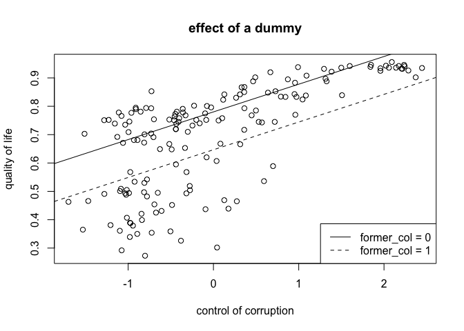
Effects of Dummies
The variable former_col is a dummy. It can take on the values 0 or 1. Such a variable does not affect the slope. It shifts the regression line. You end up with a second regression line (when the dummy is 1) parallel to the first (when the dummy is 0).
So, while continuous variables affect the slope, binary variables affect the intercept.
# we remove NA's
world.data <- na.omit(world.data)
# run the multiple regression
m1 <- lm(undp_hdi ~ wbgi_cce + former_col, data = world.data)
# regression table
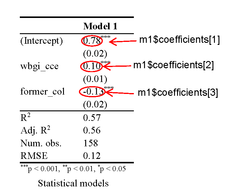
screenreg(m1)
=======================
             Model 1
-----------------------
(Intercept)    0.78 ***
              (0.02)
wbgi_cce       0.10 ***
              (0.01)
former_col    -0.13 ***
              (0.02)
-----------------------
R^2            0.57
Adj. R^2       0.56
Num. obs.    158
RMSE           0.12
=======================
*** p < 0.001, ** p < 0.01, * p < 0.05
The effect of a dummy
| Value of the dummy | Where line intercepts y-axis | Slope |
|---|---|---|
| 0 (not a former colony) | intercept + dummy coefficient * 0 | coefficient of control of corruption |
| 0.78 + (-0.13) * 0 | 0.10 | |
| 1 (was colonized) | intercept + dummy coefficient * 1 | coefficient of control of corruption |
| 0.78 + (-0.13) * 1 | 0.10 |
To illustrate the effect of a dummy we need to access the coefficients of our lm model directly. We can do this like so:
# look at cofficients of m1
m1$coefficients
(Intercept)    wbgi_cce  former_col
 0.78021162  0.09769371 -0.13352132
Subsetting lets us access individual coefficients.
You can abbreviate as well, using m1$coeff[1] for example.
To illustrate the effect of a dummy we draw a scatterplot and then use abline() to draw our regression lines within the plot. You can directly pass an intercept and a slope to abline using coef() inside it. In the table above we see that the slope remains the same. The intercept however changes. Let's draw this using: abline(coef = c(intercept, slope)). We call our regression coefficients using m1$coeffients[position of coefficient].
# scatter plot
plot(undp_hdi ~ wbgi_cce, data = world.data,
     xlab = "control of corruption",
     ylab = "quality of life",
     main = "effect of a dummy")

# the regression line when former_col = 0
abline(coef = c(m1$coefficients[1], m1$coefficients[2]), lty = "solid")

# the regression line when former_col = 1
abline(coef = c(m1$coefficients[1] + m1$coefficients[3], m1$coefficients[2]), lty = "dashed")

# add a legend to the plot
legend("bottomright", c("former_col = 0", "former_col = 1"), lty = c("solid", "dashed"))
Interactions: continuous and binary
We interact control of corruption (continuous) with having been colonized (binary). We estimate the standard model without interaction and the model including the interaction in zelig(). We use the F-test to see whether our new model does better than the simple model. It does.
| What to keep in mind when modelling interactions | |
|---|---|
 |
Include interaction terms and constituents of the interaction in your model. |
| Interaction | wbgi_cce:former_col |
| Constituent 1 | wbgi_cce |
| Constituent 2 | former_col |
# first model
z.out1 <- zelig(undp_hdi ~ wbgi_cce + former_col,
                model = "ls", data = world.data, cite = FALSE)
# second model
z.out2 <- zelig(undp_hdi ~ wbgi_cce + former_col + wbgi_cce:former_col,
                model = "ls", data = world.data, cite = FALSE)

# F-test (see seminar 5)
anova(z.out1$result, z.out2$result)
Analysis of Variance Table

Model 1: undp_hdi ~ wbgi_cce + former_col
Model 2: undp_hdi ~ wbgi_cce + former_col + wbgi_cce:former_col
  Res.Df    RSS Df Sum of Sq      F  Pr(>F)
1    155 2.3318
2    154 2.2269  1   0.10499 7.2607 0.00783 **
---
Signif. codes:  0 '***' 0.001 '**' 0.01 '*' 0.05 '.' 0.1 ' ' 1
# regression table
screenreg(list(z.out1, z.out2))
=============================================
                     Model 1      Model 2
---------------------------------------------
(Intercept)             0.78 ***     0.79 ***
                       (0.02)       (0.02)
wbgi_cce                0.10 ***     0.07 ***
                       (0.01)       (0.01)
former_col             -0.13 ***    -0.13 ***
                       (0.02)       (0.02)
wbgi_cce:former_col                  0.06 **
                                    (0.02)
---------------------------------------------
AIC                  -209.73      -215.01
BIC                  -197.48      -199.70
Log Likelihood        108.87       112.51
Num. obs.             158          158
R^2                     0.57         0.59
Adj. R^2                0.56         0.58
F statistic           101.71        72.97
=============================================
*** p < 0.001, ** p < 0.01, * p < 0.05
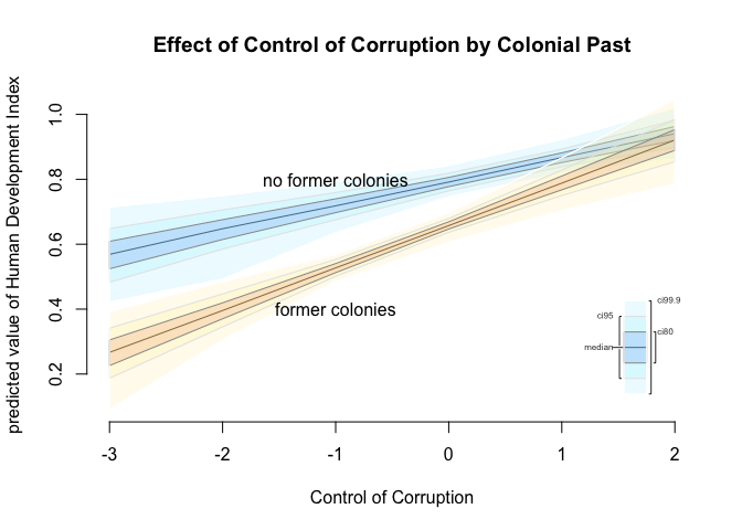
We now examine what our interaction in z.out2 does. First, we compare intercept and slope coefficients conditional on whether a country was colonized or not. Second, we plot our results using zelig().
Comparing Intercepts and Slopes
We can access coefficients of a zelig object like so: name.of.object$res$coeff. We can subset this to get the first, second or nth coefficients respectively using square brackets.
Remember, binary variables affect the intercept. Continuous variables affect the slope.
| Value of the dummy | Intercept | Slope |
|---|---|---|
| 0 | intercept coefficient | slope coefficient (of continuous variable) |
| 1 | intercept + dummy coefficient | slope coefficient (of continuous variable) + interaction coefficient |
# intercepts and slopes of control of corruption
intercepts <- c(z.out2$res$coeff[1], z.out2$res$coeff[1] + z.out2$res$coeff[3])
slopes <- c(z.out2$res$coeff[2], z.out2$res$coeff[2] + z.out2$res$coeff[4])

# rbind combines separate vectors or matrices or data frames row-wise
cond.efcts <- rbind(intercepts,slopes)

# colnames lets you define names of columns of a matrix like object
colnames(cond.efcts) <- c("never colony", "former colony")

# lets examine the effects
# the function round lets us round to 2 digits
round(cond.efcts, digits = 2)
           never colony former colony
intercepts         0.79          0.66
slopes             0.07          0.13
Ploting our results
We will plot our results using simulation in zelig(). The first scenario x.out1 represents countries that were never colonized. The second, x.out2 represents former colonies. We vary control of corruption from -3 to 2 which is roughly the minimum to the maximum of the variable.
Note: We did na.omit(world.data) earlier. You will run into problems with zelig if your data contains missings. Here, the plot will not work. To be safe remove missings before you get to this stage.
# set covariates for countries that weren't colonised
x.out1 <- setx(z.out2, former_col = 0, wbgi_cce = -3:2)

# set covariates for colonised countries
x.out2 <- setx(z.out2, former_col = 1, wbgi_cce = -3:2)

# simulate
s.out <- sim(z.out2, x = x.out1, x1 = x.out2)

# plot results
# you will run into problems here if you forgot to do na.omit(world.data)
plot(s.out,
     xlab = "Control of Corruption",
     ylab = "predicted value of Human Development Index",
     main = "Effect of Control of Corruption by Colonial Past"
    )

# add text to Zelig plot where x and y are plot coordinates
text( x = -1, y = .8, labels = "no former colonies")
text( x = -1, y = .4, labels = "former colonies")
Interactions: two continuous variables
When looking at the scatter plot, we clearly see a non-linear relationship between the x-variable (GDP/captia) and the y-variable (quality of life.). We fit a linear line through the point cloud using abline(). You see that points below $5000 and above $35,000 are below the line while points in between are above the line. This goes along well with our intuition. Additional wealth has a large effect on the quality of life in a poor country while the effect becomes smaller and smaller when higher levels of wealth are reached. That, however, implies that the slope of our line (the effect of the independent variable) should depend on the level of the independent variable.
# we check min and max of variables of interest to draw plot limits (xlim & ylim)
summary(world.data[, c("undp_hdi", "wdi_gdpc")  ])
    undp_hdi         wdi_gdpc
 Min.   :0.2730   Min.   :  226.2
 1st Qu.:0.5218   1st Qu.: 1735.0
 Median :0.7455   Median : 5493.4
 Mean   :0.6947   Mean   :10702.0
 3rd Qu.:0.8370   3rd Qu.:14516.8
 Max.   :0.9560   Max.   :63686.7
# plot of relationship b/w income & the human development index
plot( undp_hdi ~ wdi_gdpc,
      data = world.data,
      xlim = c( xmin = 0, xmax = 65000),
      ylim = c( ymin = 0, ymax = 1),
      frame = FALSE,
      xlab = "World Bank GDP/captia",
      ylab = "Human Development Index",
      main = "Relationship b/w Income and Quality of Life")

# add the regression line using zelig() within abline()
abline(zelig(undp_hdi ~ wdi_gdpc, data = world.data, model = "ls", cite = FALSE))

# lowess line
lines(lowess(world.data$wdi_gdpc, world.data$undp_hdi), col="red")
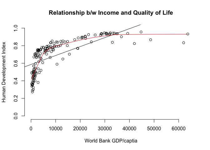
We can model such a non-linear relationship by including a quadratic term of GDP per captia. Have a look at the shape of a quadratic function to see why. Below we include a quadratic term. The syntax is the following: I(independent_variable^2).
| Component | Meaning |
|---|---|
I |
The capital I before the opening parenthesis means "as is" and tells Zelig to include the quadratic term as we calculate it and estimate parameters for both terms (interaction AND constituent). |
^2 |
The hat followed by a 2 means: to the power of two. |
# we include a quadradic term for income
z.out <- zelig(undp_hdi ~ wdi_gdpc + I(wdi_gdpc^2),
               data = world.data, model = "ls", cite = FALSE)

# regression output
summary(z.out)
Call:
lm(formula = formula, weights = weights, model = F, data = data)

Residuals:
      Min        1Q    Median        3Q       Max
-0.261986 -0.070042 -0.003689  0.090414  0.222661

Coefficients:
                Estimate Std. Error t value Pr(>|t|)
(Intercept)    5.202e-01  1.305e-02  39.856   <2e-16 ***
wdi_gdpc       2.549e-05  1.777e-06  14.345   <2e-16 ***
I(wdi_gdpc^2) -3.534e-10  3.815e-11  -9.264   <2e-16 ***
---
Signif. codes:  0 '***' 0.001 '**' 0.01 '*' 0.05 '.' 0.1 ' ' 1

Residual standard error: 0.1059 on 155 degrees of freedom
Multiple R-squared:  0.6776,    Adjusted R-squared:  0.6734
F-statistic: 162.9 on 2 and 155 DF,  p-value: < 2.2e-16
# do we need the quadratic term or is the relationship in fact linear?
# use an F-Test to check
z.out.base <- zelig(undp_hdi ~ wdi_gdpc, data = world.data, model = "ls", cite = FALSE)
anova(z.out.base$res, z.out$res)
Analysis of Variance Table

Model 1: undp_hdi ~ wdi_gdpc
Model 2: undp_hdi ~ wdi_gdpc + I(wdi_gdpc^2)
  Res.Df    RSS Df Sum of Sq      F    Pr(>F)
1    156 2.7010
2    155 1.7384  1   0.96263 85.831 < 2.2e-16 ***
---
Signif. codes:  0 '***' 0.001 '**' 0.01 '*' 0.05 '.' 0.1 ' ' 1
# setting covariates; GDP/captia is a sequence from 0 to 45000 by steps of 1000
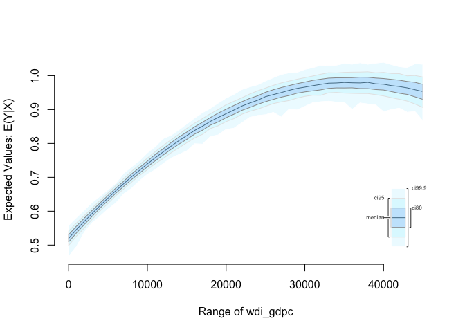
x.out <- setx(z.out, wdi_gdpc = seq(0, 45000, 1000))
# simulate using our model and our covariates
s.out <- sim(z.out, x = x.out)
# plot the results
plot(s.out)
Dplyr arrange()
On some occasions you might want to order a data set according to several criteria. arrange() from dplyr let's you do that. The default order is ascending. To change to descending, use desc().
# we order by ex-colony and then hdi
head(arrange(world.data, former_col, undp_hdi))
  h_j  wdi_gdpc undp_hdi    wbgi_cce   wbgi_pse former_col lp_lat_abst
1   1  550.5092    0.359 -0.50416088 -1.3376564          0   0.0888889
2  -5  907.1852    0.504 -0.27502340 -1.5360656          0   0.3111111
3   1 2140.4829    0.668  0.08207824  1.0622551          0   0.5111111
4  -5 1178.8358    0.671 -1.06050229 -1.3677230          0   0.4333333
5   1 1904.1436    0.681 -0.93192887 -0.1513168          0   0.5222222
6  -5 1556.3955    0.701 -0.80801731 -1.0340041          0   0.4555556
# note: to change the data set you would have to assign it:
# world.data <- arrange(world.data, former_col, undp_hdi)

# the default order is ascending, for descending use:
head(arrange(world.data, desc(former_col, undp_hdi)))
  h_j   wdi_gdpc undp_hdi   wbgi_cce   wbgi_pse former_col lp_lat_abst
1  -5  6349.7207    0.704 -0.7301510 -1.7336243          1   0.3111111
2  -5  2856.7517    0.381 -1.2065741 -1.4150945          1   0.1366667
3  -5  8584.8857    0.853 -0.7264611 -1.0361214          1   0.3777778
4  -5 24506.4883    0.843  0.9507225  0.2304108          1   0.2888889
5  -5   947.5254    0.509 -1.0845362 -0.8523579          1   0.2666667
6   1 19188.6406    0.888  1.3267342  1.0257839          1   0.1455556
Exercises
Using our model
z.out, where we included the square of GDP/capita, what is the effect of:- an increase of GDP/captia from 5000 to 15000?
- an increase of GDP/capita from 25000 to 35000?
Estimate a model where
wbgi_pse(political stability) is the response variable andh_j(1 if country has an independent judiciary) andformer_colare the explanatory variables. Include an interaction between your explanatory variables. What is the marginal effect of:- An independent judiciary when the country is a former colony?
- An independent judiciary when the country was not colonized?
- Does the interaction between
h_jandformer_colimprove model fit?
Run a model on the human development index (
undp_hdi), interacting an independent judiciary (h_j) and control of corruption (wbgi_cce). What is the effect of control of corruption:- In countries without an independent judiciary?
- When there is an independent judiciary?
- Illustrate your results.
- Does the interaction improve model fit?
Clear your workspace and download the California Test Score Data used in Chapters 4-9 by Stock and Watson.