- Introduction
- 1. Introduction to Quantitative Analysis
- 2. Descriptive Statistics
- 3. T-test for Difference in Means and Hypothesis Testing
- 4. Bivariate linear regression models
- 5. Multiple linear regression models
- 6. Assumptions and Violations of Assumptions
- 7. Interactions
- 8. Panel Data, Time-Series Cross-Section Models
- 9. Binary models: Logit
- 10. Frequently Asked Questions
- 11. Optional Material
- 12. Datasets
- 13. R Resources
- 14. References
- Published with GitBook
7. Interactions
7.2 Solutions
Exercise 1
Using our model z.out , where we included the square of GDP/capita, what is the effect of:
- an increase of GDP/captia from $5,000 to $15,000?
- an increase of GDP/capita from $25,000 to $35,000?
Solution
We will re-estimate the same model we had done in class. To do that we need to load foreign, texreg and Zelig libraries. We also clear our workspace and load the data set. We create a subset of the loaded data set that includes only the two variables that we need for this exercise. We do na.omit() over that subset to drop missing values but only from the variables that we include in our model.
library(foreign) # to load .dta files
library(texreg) # to print nice regression tables
Warning: package 'texreg' was built under R version 3.2.3
library(Zelig) # to model & illustrate uncertainty
# clear workspace
rm(list = ls())

# load data set from seminar page
data.set <- read.dta("http://uclspp.github.io/PUBLG100/data/QoG2012.dta")

# exercise subset
exercise.subset <- data.set[, c("undp_hdi", "wdi_gdpc")]

# removing NA's on our two variables of interest
exercise.subset <- na.omit(exercise.subset)

# running regression with squared GDP/captia
exercise1.reg <- zelig(undp_hdi ~ wdi_gdpc + I(wdi_gdpc^2), model = "ls",
                       data = exercise.subset, cite = FALSE)

screenreg(exercise1.reg)
===========================
                Model 1
---------------------------
(Intercept)        0.53 ***
                  (0.01)
wdi_gdpc           0.00 ***
                  (0.00)
I(wdi_gdpc^2)     -0.00 ***
                  (0.00)
---------------------------
AIC             -282.52
BIC             -269.93
Log Likelihood   145.26
Num. obs.        172
R^2                0.67
Adj. R^2           0.66
F statistic      170.11
===========================
*** p < 0.001, ** p < 0.01, * p < 0.05
Having done these preliminary tasks, we get to crux of the question. The model that we estimated is not linear because we included a quadratic term. The effect of a $10,000 increase on the quality of life, thus, depends on the initial level of wealth. We proceed like this:
- We use Zelig to simulate the quality of life when GDP/captia is $5,000 and when it is $15,000. Zelig takes the difference between these two values for us, called first differences. It also reports the 95% confidence interval, telling us whether we can say that the difference is statistically significant.
- We use Zelig to do the same thing again but this time for GDP/captia values of $25,000 and $35,000. Again, we see whether the difference is statistically significant.
- The differences are the effects of increasing GDP/captia by $10,000, taking the initial level of wealth into account. We compare how large the differences are in relation to the range of the dependent variable, to say whether the effect is large or small.
## effect of an increase from $5,000 to $15,000
# set.seed() makes your results replicable, it does not
# matter which values you put inside
set.seed(123)

# setting covariates
set.gdp5000 <- setx(exercise1.reg, wdi_gdpc = 5000)
set.gdp15000 <- setx(exercise1.reg, wdi_gdpc = 15000)

# simulating
sim.5000.to.15000 <- sim(exercise1.reg, x = set.gdp5000, x1 = set.gdp15000)

# checking for the first differences
summary(sim.5000.to.15000)
Model:  ls
Number of simulations:  1000

Values of X
  (Intercept) wdi_gdpc I(wdi_gdpc^2)
2           1     5000       2.5e+07
attr(,"assign")
[1] 0 1 2

Values of X1
  (Intercept) wdi_gdpc I(wdi_gdpc^2)
2           1    15000      2.25e+08
attr(,"assign")
[1] 0 1 2

Expected Values: E(Y|X)
   mean    sd   50%  2.5% 97.5%
2 0.644 0.008 0.644 0.628 0.661

Expected Values: E(Y|X1)
   mean    sd   50%  2.5% 97.5%
2 0.827 0.012 0.826 0.804 0.851

Predicted Values: Y|X
   mean    sd   50%  2.5% 97.5%
2 0.644 0.008 0.644 0.628 0.661

Predicted Values: Y|X1
   mean    sd   50%  2.5% 97.5%
2 0.827 0.012 0.826 0.804 0.851

First Differences: E(Y|X1) - E(Y|X)
   mean    sd   50%  2.5% 97.5%
2 0.182 0.011 0.182 0.161 0.204
## effect of an increase from 25,000 to 35,000
# setting covariates
set.gdp25000 <- setx(exercise1.reg, wdi_gdpc = 25000)
set.gdp35000 <- setx(exercise1.reg, wdi_gdpc = 35000)

# simulating
sim.25000.to.35000 <- sim(exercise1.reg, x = set.gdp25000, x1 = set.gdp35000)

# checking for the first differences
summary(sim.25000.to.35000)
Model:  ls
Number of simulations:  1000

Values of X
  (Intercept) wdi_gdpc I(wdi_gdpc^2)
2           1    25000      6.25e+08
attr(,"assign")
[1] 0 1 2

Values of X1
  (Intercept) wdi_gdpc I(wdi_gdpc^2)
2           1    35000     1.225e+09
attr(,"assign")
[1] 0 1 2

Expected Values: E(Y|X)
  mean    sd  50%  2.5% 97.5%
2 0.94 0.015 0.94 0.909  0.97

Expected Values: E(Y|X1)
   mean    sd   50%  2.5% 97.5%
2 0.981 0.018 0.981 0.947 1.014

Predicted Values: Y|X
  mean    sd  50%  2.5% 97.5%
2 0.94 0.015 0.94 0.909  0.97

Predicted Values: Y|X1
   mean    sd   50%  2.5% 97.5%
2 0.981 0.018 0.981 0.947 1.014

First Differences: E(Y|X1) - E(Y|X)
   mean    sd   50%  2.5% 97.5%
2 0.041 0.009 0.042 0.024 0.059
# checking summary statistics of wealth
summary(exercise.subset$wdi_gdpc)
   Min. 1st Qu.  Median    Mean 3rd Qu.    Max.
  226.2  1776.0  5493.0 10420.0 13840.0 63690.0
# checking 25th percentile and 75th percentile
quantile(exercise.subset$wdi_gdpc, probs = c(0.25, 0.75))
      25%       75%
 1776.097 13837.955
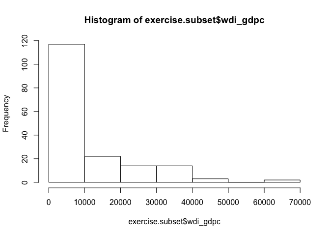
# looking at the distribution of wealth
hist(exercise.subset$wdi_gdpc)
# checking summary statistic of the dependent variable
summary(exercise.subset$undp_hdi)
   Min. 1st Qu.  Median    Mean 3rd Qu.    Max.
 0.2730  0.5355  0.7505  0.6978  0.8350  0.9560
diff(range(exercise.subset$undp_hdi))
[1] 0.683
# the effect of increasing from $5000 to $15000
summary(sim.5000.to.15000)
Model:  ls
Number of simulations:  1000

Values of X
  (Intercept) wdi_gdpc I(wdi_gdpc^2)
2           1     5000       2.5e+07
attr(,"assign")
[1] 0 1 2

Values of X1
  (Intercept) wdi_gdpc I(wdi_gdpc^2)
2           1    15000      2.25e+08
attr(,"assign")
[1] 0 1 2

Expected Values: E(Y|X)
   mean    sd   50%  2.5% 97.5%
2 0.644 0.008 0.644 0.628 0.661

Expected Values: E(Y|X1)
   mean    sd   50%  2.5% 97.5%
2 0.827 0.012 0.826 0.804 0.851

Predicted Values: Y|X
   mean    sd   50%  2.5% 97.5%
2 0.644 0.008 0.644 0.628 0.661

Predicted Values: Y|X1
   mean    sd   50%  2.5% 97.5%
2 0.827 0.012 0.826 0.804 0.851

First Differences: E(Y|X1) - E(Y|X)
   mean    sd   50%  2.5% 97.5%
2 0.182 0.011 0.182 0.161 0.204
# calculating the effect in percentage terms (compared to the range of DV)
0.182 / diff(range(exercise.subset$undp_hdi))
[1] 0.2664715
# the effect of increasing from $25000 to $35000
summary(sim.25000.to.35000)
Model:  ls
Number of simulations:  1000

Values of X
  (Intercept) wdi_gdpc I(wdi_gdpc^2)
2           1    25000      6.25e+08
attr(,"assign")
[1] 0 1 2

Values of X1
  (Intercept) wdi_gdpc I(wdi_gdpc^2)
2           1    35000     1.225e+09
attr(,"assign")
[1] 0 1 2

Expected Values: E(Y|X)
  mean    sd  50%  2.5% 97.5%
2 0.94 0.015 0.94 0.909  0.97

Expected Values: E(Y|X1)
   mean    sd   50%  2.5% 97.5%
2 0.981 0.018 0.981 0.947 1.014

Predicted Values: Y|X
  mean    sd  50%  2.5% 97.5%
2 0.94 0.015 0.94 0.909  0.97

Predicted Values: Y|X1
   mean    sd   50%  2.5% 97.5%
2 0.981 0.018 0.981 0.947 1.014

First Differences: E(Y|X1) - E(Y|X)
   mean    sd   50%  2.5% 97.5%
2 0.041 0.009 0.042 0.024 0.059
# calculating the effect in percentage (compared to range of DV)
0.041 / diff(range(exercise.subset$undp_hdi))
[1] 0.06002929
We have all we need for statistical and substantial interpretation. Suppose, someone claims that the quality of life depends on how wealthy a society is. What is more, (s)he also claims that added wealth increases quality of life independent of how wealthy a society is.
To check - with the goal of disproving - we look at the relationship between a societies wealth (GDP/captia) and the quality of life in a scatter plot. From that we already got a very clear idea that the relationship is in fact not linear. To be sure, we estimated a regression model including a quadratic term of GDP/captia. We find that the interaction (GDP/captia times GDP/captia) is statistically significant, therefore disproving the claim that the effect of added wealth is independent of initial wealth.
Our friend looks at our results and says that the coefficients are extremely small and that therefore our findings have no substantial meaning in the real world. We know that the effect is larger for poorer societies than for richer societies but how big is it? We estimate the effect of a large leap in GDP/capita of $10,000 for different initial wealth levels.
Our results show that quality of life increases by 0.182 when increasing GDP/capita from 5,000 to 15,000. That is a change of 27% of the entire range of the quality of life measure. The effect is huge. Wealth matters a lot in poorer societies. A move from $5,000 of GDP/captia to $15,000 is no small feat however. Half the countries in our sample have a GDP/capita that is lower than $5,500 and a wealth level of $15,000 means that more than 75% of the countries are poorer.
To show that the effect of wealth levels out we consider what happens when moving from being a rich country to a super rich country (GDP/captia from $25,000 to $35,000). We predict a mean increase in the quality of life index of 0.041 (on a 95% level between 0.024 and 0.059). That still corresponds to an increase of 6% in of the range of quality of life. That is still a very large effect. However, we must admit that an increase of $10,000 in GDP/captia is huge as well.
Note: This way of interpreting the effect relies on comparing the effect for a change of X to the range of Y in the sample.
Exercise 2
Estimate a model where wbgi_pse (political stability) is the response variable and h_j (1 if country has an independent judiciary) and former_col are the explanatory variables. Include an interaction between your explanatory variables. What is the marginal effect of:
- An independent judiciary when the country is a former colony?
- An independent judiciary when the country was not colonized?
- Does the interaction between
h_jand former_col improve model fit?
We clear our workspace again. Then we reload the data set and create a subset that only includes the variables that we care about. We then remove missing values from that subset. We estimate the two models and compare the results.
Solution
# clear workspace
rm(list = ls())

# load data set
data.set <- read.dta("http://uclspp.github.io/PUBLG100/data/QoG2012.dta")

# subset for analysis
exercise2.subset <- data.set[, c("wbgi_pse", "h_j", "former_col")]

# remove missings from subset
exercise2.subset <- na.omit(exercise2.subset)

# estimate model without interaction
base.model <- zelig(wbgi_pse ~ h_j + former_col, model = "ls",
                    data = exercise2.subset, cite = FALSE)

# estimate model including the interaction
interaction.model <- zelig(wbgi_pse ~ h_j + former_col + h_j*former_col,
                           model = "ls", data = exercise2.subset, cite = FALSE)

# comparing the models
screenreg(list(base.model, interaction.model))
========================================
                Model 1      Model 2
----------------------------------------
(Intercept)        0.39 ***     0.47 ***
                  (0.11)       (0.11)
h_j                0.17 ***     0.24 ***
                  (0.03)       (0.04)
former_col        -0.16        -0.49 *
                  (0.15)       (0.19)
h_j:former_col                 -0.14 **
                               (0.05)
----------------------------------------
AIC              432.32       426.69
BIC              444.83       442.34
Log Likelihood  -212.16      -208.34
Num. obs.        169          169
R^2                0.28         0.31
Adj. R^2           0.27         0.30
F statistic       32.53        25.09
========================================
*** p < 0.001, ** p < 0.01, * p < 0.05
# F-test
anova(base.model$result, interaction.model$result)
Analysis of Variance Table

Model 1: wbgi_pse ~ h_j + former_col
Model 2: wbgi_pse ~ h_j + former_col + h_j * former_col
  Res.Df    RSS Df Sum of Sq      F   Pr(>F)
1    166 121.85
2    165 116.47  1    5.3762 7.6163 0.006438 **
---
Signif. codes:  0 '***' 0.001 '**' 0.01 '*' 0.05 '.' 0.1 ' ' 1
Policy experts are interested in the political stability of a country. They conjecture that the existence of an independent judiciary is important, i.e. countries that have one are more stable than those that do not. They also claim that whether a country was colonised or not does not make a difference. A new theory, however, claims that the effect of an independent judiciary depends on whether a country was colonised or not. We test this new theory against the old one.
Model 1 represents the conventional theory. Indeed, we find that countries with an independent judiciary are more stable than those without. And in addition, there is no difference in political stability between countries that have been colonised and those that have not been.
Model 2 represents the more refined theory. The interaction is significant and the F-test is significant as well, indicating that our new model does better at explaining political stability. And the new theory is right, the effect of an independent judiciary is conditional on whether a country was colonised or not.
The model is linear, we get the effect of an independent judiciary when a country was not colonised directly from model 2 in our table. The difference between countries with an independent judiciary and without conditional on not having been colonised is 0.24 on the political stability scale (the effect of the dummy h_j). The difference that having an independent judiciary makes for countries that have been colonised is smaller. It is 0.10 on the political stability scale (the effect of the dummy h_j plus the effect of the interaction).
Are those differences large or small?
# summary statistics of the dependent variable
summary(exercise2.subset$wbgi_pse)
   Min. 1st Qu.  Median    Mean 3rd Qu.    Max.
-2.4670 -0.8114 -0.1550 -0.1655  0.6775  1.6760
# range of the dependnet variable
diff(range(exercise2.subset$wbgi_pse))
[1] 4.14307
# percentage change in pol. stability of having indep. judiciary if NOT colonised
0.24 / diff(range(exercise2.subset$wbgi_pse))
[1] 0.05792806
# percentage change in pol. stability of having indep. judiciary if colonised
0.10 / diff(range(exercise2.subset$wbgi_pse))
[1] 0.02413669
Those countries that have an independent judiciary and that were not colonised are 6% more stable (compared to the range of the political stability scale as observed in the sample) than those without an independent judiciary. Having an independent judiciary makes a difference of 2% if the country was colonised. Those differences are not very large. However, given that political stability is paramount, having an independent judiciary is a good idea. It makes less of a difference in countries that have been colonised. We should be aware that these theories are quite rudimentary and that we may have omitted causes.
Note: The interpretation, relies on finding the differences between the groups as we only have dummies in the model. The size of the differences again relies on comparing the difference that X makes to the range of Y.
Exercise 3
Run a model on the human development index (undp_hdi), interacting an independent judiciary (h_j) and control of corruption (wbgi_cce). What is the effect of control of corruption:
- In countries without an independent judiciary?
- When there is an independent judiciary?
- Illustrate your results.
- Does the interaction improve model fit?
Solution
We clear our workspace, reload the data set and create a subset that includes only the variables that we care about. We drop missings from this subset. We estimate the two models. We then compare the regression tables and we do an F-test.
# clear workspace
rm(list = ls())

# load data set
data.set <- read.dta("http://uclspp.github.io/PUBLG100/data/QoG2012.dta")

# subset for analysis
exercise3.subset <- data.set[, c("undp_hdi", "h_j", "wbgi_cce")]

# remove missings
exercise3.subset <- na.omit(exercise3.subset)

# estimate model without interaction
base.model <- zelig(undp_hdi ~ wbgi_cce + h_j, model = "ls", data = exercise3.subset,
                    cite = FALSE)

# estimate interaction model
interaction.model <- zelig(undp_hdi ~ wbgi_cce + h_j + wbgi_cce:h_j,
                           model = "ls", data = exercise3.subset, cite = FALSE)

# output table
screenreg(list(base.model, interaction.model))
========================================
                Model 1      Model 2
----------------------------------------
(Intercept)        0.72 ***     0.72 ***
                  (0.02)       (0.02)
wbgi_cce           0.11 ***     0.11 ***
                  (0.01)       (0.01)
h_j                0.01         0.01
                  (0.00)       (0.00)
wbgi_cce:h_j                    0.00
                               (0.00)
----------------------------------------
AIC             -183.41      -181.61
BIC             -171.11      -166.23
Log Likelihood    95.70        95.80
Num. obs.        160          160
R^2                0.48         0.48
Adj. R^2           0.47         0.47
F statistic       71.90        47.75
========================================
*** p < 0.001, ** p < 0.01, * p < 0.05
# F-Test
anova(base.model$result, interaction.model$result)
Analysis of Variance Table

Model 1: undp_hdi ~ wbgi_cce + h_j
Model 2: undp_hdi ~ wbgi_cce + h_j + wbgi_cce:h_j
  Res.Df    RSS Df Sum of Sq      F Pr(>F)
1    157 2.8320
2    156 2.8285  1 0.0035607 0.1964 0.6583
Comparing the two models we see that there is an effect of control of corruption on the quality of life. The better the institutions (more control of corruption), the higher the quality of life. We test the theory that the effect of control of corruption is conditional on having an independent judiciary, i.e. the magnitude of the effect is different in the two sub-groups. Our interaction term is insignificant. The effect of control of corruption seems to be independent of whether an independent judiciary exists or not. Our F-test also clearly rejects that our model with the interaction is doing better at explaining quality of life (as do AIC and BIC).
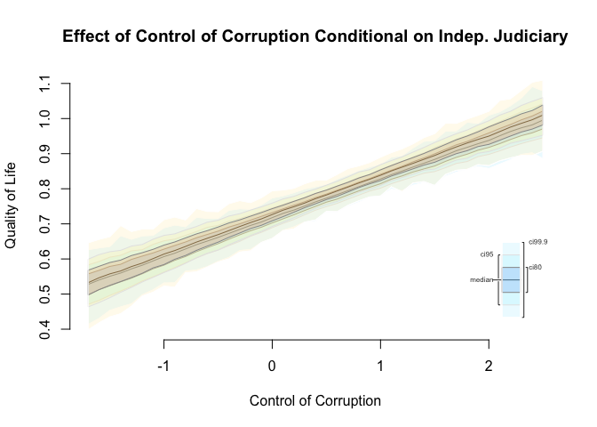
Normally, we would stop here. There is no point in illustrating a conditional effect that does not exist. However, below we illustrate the effect of control of corruption conditional on having an independent judiciary. The effects overlap and we cannot tell a difference.
Note: The interpretation relies on statistical significance. We do not find support for the conditional effect of X on Y.
# illustration of results

# range of control of corruption
summary(exercise3.subset$wbgi_cce)
    Min.  1st Qu.   Median     Mean  3rd Qu.     Max.
-1.70000 -0.83960 -0.32230 -0.02757  0.57480  2.44600
# setting the two scenarios
no.indep.jud.setx <- setx(interaction.model, h_j = 0, wbgi_cce = seq(-1.7, 2.5, 0.1) )
an.indep.jud.setx <- setx(interaction.model, h_j = 1, wbgi_cce = seq(-1.7, 2.5, 0.1) )

# simulation
simulation.result <- sim(interaction.model, x = no.indep.jud.setx, x1 = an.indep.jud.setx)

# plot results
plot(simulation.result,
     main = "Effect of Control of Corruption Conditional on Indep. Judiciary",
     xlab = "Control of Corruption",
     ylab = "Quality of Life")
Exercise 4
Clear your workspace and download the California Test Score Data used in Chapters 4-9 by Stock and Watson.
- Draw a scatter plot between district income and test scores.
- Run two regressions. One with and one without quadratic income.
- Test whether the quadratic model fits the data better.
Solution
# clear workspace
rm(list = ls())

# load data set from your local folder where you saved the data set
california.schools <- read.dta("caschool.dta")

# check variable names
names(california.schools)
 [1] "observat" "dist_cod" "county"   "district" "gr_span"  "enrl_tot"
 [7] "teachers" "calw_pct" "meal_pct" "computer" "testscr"  "comp_stu"
[13] "expn_stu" "str"      "avginc"   "el_pct"   "read_scr" "math_scr"
# summary stats of variables of interest
summary(california.schools[, c("testscr", "avginc")])
    testscr          avginc
 Min.   :605.5   Min.   : 5.335
 1st Qu.:640.0   1st Qu.:10.639
 Median :654.5   Median :13.728
 Mean   :654.2   Mean   :15.317
 3rd Qu.:666.7   3rd Qu.:17.629
 Max.   :706.8   Max.   :55.328
# checking for missings in data set
summary(california.schools)
    observat        dist_cod        county            district
 Min.   :  1.0   Min.   :61382   Length:420         Length:420
 1st Qu.:105.8   1st Qu.:64308   Class :character   Class :character
 Median :210.5   Median :67760   Mode  :character   Mode  :character
 Mean   :210.5   Mean   :67473
 3rd Qu.:315.2   3rd Qu.:70419
 Max.   :420.0   Max.   :75440
   gr_span             enrl_tot          teachers          calw_pct
 Length:420         Min.   :   81.0   Min.   :   4.85   Min.   : 0.000
 Class :character   1st Qu.:  379.0   1st Qu.:  19.66   1st Qu.: 4.395
 Mode  :character   Median :  950.5   Median :  48.56   Median :10.520
                    Mean   : 2628.8   Mean   : 129.07   Mean   :13.246
                    3rd Qu.: 3008.0   3rd Qu.: 146.35   3rd Qu.:18.981
                    Max.   :27176.0   Max.   :1429.00   Max.   :78.994
    meal_pct         computer         testscr         comp_stu
 Min.   :  0.00   Min.   :   0.0   Min.   :605.5   Min.   :0.00000
 1st Qu.: 23.28   1st Qu.:  46.0   1st Qu.:640.0   1st Qu.:0.09377
 Median : 41.75   Median : 117.5   Median :654.5   Median :0.12546
 Mean   : 44.71   Mean   : 303.4   Mean   :654.2   Mean   :0.13593
 3rd Qu.: 66.86   3rd Qu.: 375.2   3rd Qu.:666.7   3rd Qu.:0.16447
 Max.   :100.00   Max.   :3324.0   Max.   :706.8   Max.   :0.42083
    expn_stu         str            avginc           el_pct
 Min.   :3926   Min.   :14.00   Min.   : 5.335   Min.   : 0.000
 1st Qu.:4906   1st Qu.:18.58   1st Qu.:10.639   1st Qu.: 1.941
 Median :5215   Median :19.72   Median :13.728   Median : 8.778
 Mean   :5312   Mean   :19.64   Mean   :15.317   Mean   :15.768
 3rd Qu.:5601   3rd Qu.:20.87   3rd Qu.:17.629   3rd Qu.:22.970
 Max.   :7712   Max.   :25.80   Max.   :55.328   Max.   :85.540
    read_scr        math_scr
 Min.   :604.5   Min.   :605.4
 1st Qu.:640.4   1st Qu.:639.4
 Median :655.8   Median :652.5
 Mean   :655.0   Mean   :653.3
 3rd Qu.:668.7   3rd Qu.:665.9
 Max.   :704.0   Max.   :709.5
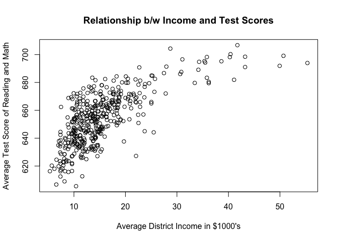
# scatter plot
plot( testscr ~ avginc, data = california.schools,
      main = "Relationship b/w Income and Test Scores",
      xlab = "Average District Income in $1000's",
      ylab = "Average Test Score of Reading and Math")
# regression exluding squared income
base.reg <- zelig( testscr ~ avginc, model = "ls", data = california.schools,
                   cite = FALSE)

# regression including squared income
square.reg <- zelig( testscr ~ avginc + I(avginc^2), model = "ls",
                     data = california.schools, cite = FALSE)

# regression tables
screenreg(list(base.reg, square.reg))
==========================================
                Model 1       Model 2
------------------------------------------
(Intercept)       625.38 ***    607.30 ***
                   (1.53)        (3.05)
avginc              1.88 ***      3.85 ***
                   (0.09)        (0.30)
I(avginc^2)                      -0.04 ***
                                 (0.01)
------------------------------------------
AIC              3375.07       3333.42
BIC              3387.19       3349.58
Log Likelihood  -1684.54      -1662.71
Num. obs.         420           420
R^2                 0.51          0.56
Adj. R^2            0.51          0.55
F statistic       430.83        261.28
==========================================
*** p < 0.001, ** p < 0.01, * p < 0.05
# F-test
anova(base.reg$result, square.reg$result)
Analysis of Variance Table

Model 1: testscr ~ avginc
Model 2: testscr ~ avginc + I(avginc^2)
  Res.Df   RSS Df Sum of Sq      F    Pr(>F)
1    418 74905
2    417 67510  1    7394.9 45.677 4.713e-11 ***
---
Signif. codes:  0 '***' 0.001 '**' 0.01 '*' 0.05 '.' 0.1 ' ' 1
An activist claims that inequality of opportunities determines test scores of pupils. Pupils from rich districts do better than pupils from poor districts. In addition, (s)he claims that one should concentrate on improving conditions in poor districts because there the effect of wealth on test scores is largest.
To test these claims, we must find out whether there is any effect of wealth on test scores at all. Second, whether that effect is non-linear, i.e. the effect of added wealth is larger for poorer districts and then levels off. And third, assuming these effects are statistically significant, we must show whether they are substantial.
To test for the effect of wealth and the non-linearity, we estimate our two models. Average district income is statistically significant. Pupils from richer districts do better. Our quadratic term is significant and has the expected sign. Thus, the effect is stronger for poorer districts and smaller for richer districts. The F-test confirms that our non-linear model does better at explaining test scores.
# descriptive summary statistics of district income
summary(california.schools$avginc)
   Min. 1st Qu.  Median    Mean 3rd Qu.    Max.
  5.335  10.640  13.730  15.320  17.630  55.330
# what is the income in the 10th percentile?
low1 <- quantile(california.schools$avginc, 0.10)
low1
     10%
8.929933
# what is the income in the 15th percentile
low2 <- quantile(california.schools$avginc, 0.15)
low2
   15%
9.7702
# how big is difference in terms of money
low2 - low1
     15%
0.840267
# illustrating effect of a move from the 10th to the 15th percentile
x.out.low1 <- setx(square.reg, avginc = low1)
x.out.low2 <- setx(square.reg, avginc = low2)

# simulation
s.out.low <- sim(square.reg, x = x.out.low1, x1 = x.out.low2)

# check first difference
summary(s.out.low)
Model:  ls
Number of simulations:  1000

Values of X
  (Intercept)   avginc I(avginc^2)
1           1 8.929933     79.7437
attr(,"assign")
[1] 0 1 2

Values of X1
  (Intercept) avginc I(avginc^2)
1           1 9.7702    95.45681
attr(,"assign")
[1] 0 1 2

Expected Values: E(Y|X)
     mean    sd     50%    2.5%   97.5%
1 638.306 1.009 638.309 636.406 640.402

Expected Values: E(Y|X1)
     mean    sd     50%    2.5%   97.5%
1 640.874 0.892 640.873 639.149 642.682

Predicted Values: Y|X
     mean    sd     50%    2.5%   97.5%
1 638.306 1.009 638.309 636.406 640.402

Predicted Values: Y|X1
     mean    sd     50%    2.5%   97.5%
1 640.874 0.892 640.873 639.149 642.682

First Differences: E(Y|X1) - E(Y|X)
   mean    sd   50%  2.5% 97.5%
1 2.568 0.163 2.567 2.231 2.878
# dependent variable summary
summary(california.schools$testscr)
   Min. 1st Qu.  Median    Mean 3rd Qu.    Max.
  605.6   640.0   654.4   654.2   666.7   706.8
# range of the depdendent variable
diff(range(california.schools$testscr))
[1] 101.2
# percent change of DV (percent change based on range of DV as observed in the sample) caused by IV
2.6 / diff(range(california.schools$testscr))
[1] 0.02569171
Following the advice of our activist and the statistically significant results of our model we check for the substantial effect of moving from the 10th percentile in district wealth to the 15th percentile. This corresponds to an increase of $840 average district income. We can show that test scores would increase by 2.6 points on average. That difference is statistically significant, we can say that on a 95% confidence level test scores would increase between 2.3 and 2.9 points. Such an increase in test scores corresponds roughly to a 3% increase in test scores (percent of range of DV as observed in the sample). That difference is quite small and may not warrant state intervention.
We also check for the effect that becoming wealthier by the same amount ($840) would have on a district from the 75th percentile.
# what is the avg. income at the 75th percentile?
high1 <- quantile(california.schools$avginc, 0.75)
high1
   75%
17.629
# we add the same amount of wealth as we did for the poor districts
high2 <- high1 + (low2 - low1)
high2
     75%
18.46927
# illustrating effect of adding $840 avg. district income to a district at 75th percentile
x.out.high1 <- setx(square.reg, avginc = high1)
x.out.high2 <- setx(square.reg, avginc = high2)

# simulation
s.out.low <- sim(square.reg, x = x.out.high1, x1 = x.out.high2)

# check first difference
summary(s.out.low)
Model:  ls
Number of simulations:  1000

Values of X
  (Intercept) avginc I(avginc^2)
1           1 17.629    310.7817
attr(,"assign")
[1] 0 1 2

Values of X1
  (Intercept)   avginc I(avginc^2)
1           1 18.46927    341.1138
attr(,"assign")
[1] 0 1 2

Expected Values: E(Y|X)
     mean    sd    50%    2.5%   97.5%
1 661.998 0.814 661.99 660.484 663.545

Expected Values: E(Y|X1)
    mean    sd     50%   2.5%   97.5%
1 663.95 0.867 663.943 662.29 665.595

Predicted Values: Y|X
     mean    sd    50%    2.5%   97.5%
1 661.998 0.814 661.99 660.484 663.545

Predicted Values: Y|X1
    mean    sd     50%   2.5%   97.5%
1 663.95 0.867 663.943 662.29 665.595

First Differences: E(Y|X1) - E(Y|X)
   mean    sd   50%  2.5% 97.5%
1 1.952 0.091 1.958 1.772 2.118
# percent change of DV (percent change based on range of DV as observed in the sample) caused by IV
2 / diff(range(california.schools$testscr))
[1] 0.01976286
When a district at the 75th percentile would become even richer by $840 average income, that would increase test scores by 2 points on average. On a 95% confidence level the increase would be in an interval from 1.8 points to 2.1 points. The increase corresponds to 2% increase of the entire range of observed test scores in our sample. That effect is smaller than in poor districts, and supports the idea that if policy intervention was taken, one should concentrate on poor districts as we would get more bang for a buck there.
Note: Here, the effect of X on Y was presented in the absolute change (point change of test scores) as well as in terms of percentage changes compared to the range of the dependent variable. When the absolute increase of the dependent variable is easy to understand it is good to do that.