12 Programming practicals

Chapter 12
Programming practicals

In this Chapter you will process some real geochronological datasets using either R or Matlab. These are both mathematical scripting languages that are both powerful and easy to use.

R is a free and open programming language that works on any operating system, including Windows, OS-X and Unix/Linux. It can be downloaded and installed from http://r-project.org.

Matlab is a proprietary programming environment. The full version of this software is very expensive but a reasonably complete student version can be purchased for £55 + VAT from http://mathworks.com. Alternatively, Octave is an open source clone of Matlab that can be downloaded for free from http://www.gnu.org/software/octave.

Sections 12.1 and 12.2 will present two brief tutorials of R and Matlab, respectively. These will cover most commands that you will need for the subsequent computer practicals.

12.1 Introduction to R

A number of different graphical user interfaces (GUIs) are available to interact with R. The most popular of these are Rgui, RStudio, RCommander and Tinn-R.

Starting these applications or running R in a text terminal presents the user with a command line prompt. Anything that is typed after the > symbol will be evaluated immediately. Thus, we can use R as a calculator:
> 1 + 1
> sqrt(2)
> exp(log(10))
> 31 %% 14
Alternatively, code can also be saved as text (using a built-in text editor) and saved as mycode.R, say. This code can then be copied and pasted at the command line prompt. Or it can be called from the command line using the source() function:
> source('mycode.R')
In the remainder of this tutorial, we will assume that your code is run from a text file unless explicitly stated otherwise. The # symbol marks the beginning of a comment. R ignores anything that follows it:
# The arrow symbol is used to assign a value to a
# variable. Note that the arrow can point both ways:
foo <- 2
4 -> bar
print(foo*bar)

# Defining a vector of multiple values:
myvec <- c(0,1,2,3,4,5)
# or, equivalently:
myvec <- seq(0,5)
# or
myvec <- seq(from=0,to=5,by=1)
# or
myvec <- 0:5

# Turn myvec into a 2x3 matrix:
mymat <- matrix(myvec,nrow=2)

# Accessing one or more elements from a vector or matrix:
x <- myvec[3]
y <- myvec[1:3]
z <- mymat[1,2:3]

# Change the third value in the second row of mymat to 10:
mymat[2,3] <- 10

# Change the entire second column of mymat to -1:
mymat[,2] <- -1

# Transpose of a matrix:
flipped <- t(mymat)

# Element-wise multiplication (*)
# vs. matrix multiplication (%*%):
rectangle <- mymat * mymat
square <- mymat %*% flipped
If you want to learn more about a function, type help() or ? at the command line prompt:
> help(c)
> ?matrix
In addition to R’s built-in functions, you can also define your own:
cube <- function(n){
    return(n^3)
}

# Using this function to take the cube of 3:
c3 <- cube(3)

# Conditional statement:
toss <- function(){
    if (runif(1)>0.5){ # runif(n) draws n random
        print("head")  # numbers between 0 and 1
    } else {
        print("tail")
    }
}

# Use a for loop to toss 10 virtual coins:
for (i in 1:10) {
    toss()
}
The purpose of the practical exercises in Sections 12.3-12.6 is to process datasets contained in external data files. For this you will need to be able to navigate through your file system and load the necessary files:
> ls() # list all the variables
> rm(list=ls()) # clear the current workspace
> getwd() # get the current working directory
> setwd("path_to_a_valid_directory")
Use the above commands to navigate to the directory containing the file named RbSr.csv. Then read this file into memory:
RbSr <- read.csv("RbSr.csv",header=TRUE)

Type names(RbSr) or colnames(RbSr) at the command prompt to list the variable names (column headers) contained in this dataset.
Let us now perform an isochron regression (Section 4.2) through these Rb-Sr data:
# Plot Sr87Sr86 against Rb87Sr86:
plot(RbSr[,'Rb87Sr86'],RbSr[,'Sr87Sr86'],type="p")

# fit a linear model to the data
fit <- lm(Sr87Sr86 ~ Rb87Sr86, data = RbSr)
fit is a ‘list’ object. Type str(fit) at the command prompt to see its structure. One of its items is fit$coefficients, which contains the slope and the intercept of the linear fit. Alternatively, we can also access these values using the coef() function. The following code uses this function to calculate the isochron age:
# define the 87Rb decay constant (in Ma-1):
lam87 <- 1.42e-5
# compute the age from the slope:
age <- log(1 + coef(fit)[2])/lam87

# predict the Sr87Sr86-ratios for the
# full range of Rb87Sr86-values:
Rb87Sr86 <- c(0,max(RbSr[,'Rb87Sr86']))
Sr87Sr86 <- coef(fit)[1] + coef(fit)[2]*Rb87Sr86

# add the predicted ratios to the existing plot:
lines(Rb87Sr86,Sr87Sr86)
# label with the isochron age:
title(age)
One of the most powerful features of R is the availability of thousands of ‘packages’ providing additional functionality to the built-in functions. For example, let us download and install the IsoplotR package from the ‘Comprehensive R Archive Network’ (CRAN):
> install.packages('IsoplotR')
We can use IsoplotR to redo the isochron regression exercise using a more rigorous weighted regression algorithm that takes into account the analytical uncertainties in both the ⁸⁷Sr/⁸⁶Sr- and ⁸⁷Rb/⁸⁶Sr-ratios:
# load the functionality of the IsoplotR package:
library('IsoplotR')

# load the data (see ?read.data for details):
RbSr2 <- read.data('RbSr.csv',method='Rb-Sr',format=1)

# compute and plot the isochron diagram:
isochron(RbSr2)

12.2 Introduction to Matlab

Matlab, like R, allows the user to run code either directly at the command line prompt, or from a built-in text editor. Anything following a percent symbol (%) is a comment and is ignored. It is considered good practice to document your code with lots of comments, as will be done in this tutorial.
% Ending a line with a semi-colon
% suppresses output to the console:
'be loud'
'stay quiet';

% Matlab can be used as a fancy calculator:
1 + 1
sqrt(2)
exp(log(10))

% Intermediate values can be stored in variables:
foo = 2;
bar = 4;
foo = foo*bar;
foo
As the name suggest, Matlab (which stands for MATrix LABoratory) is capable of, and excels at, dealing with collections of multiple numbers arranged in vectors and matrices:
% Data can be entered as vectors:
x = [0 2 4 6 8 10]
% or using shorthand syntax:
y = 0:2:10

% Define a matrix
z = [1 2 3
     4 5 6
     7 8 9];

% Accessing one or more elements
% from a matrix or vector:
x(3)
y(1:3)
z(1:2,2:3)

% Attention: '*', '/' and '^' symbols
% are reserved for matrix operations:
a = [1 1 1]  % row vector
b = [1;1;1]  % column vector
a*b

% Use '.*', './' and '.^' for
% element-wise operations:
a.*a

% Transpose of a matrix:
z'
In addition to Matlab’s built-in operators and functions, you can also define your own:
% take the cube of the input argument:
function out = cube(in)
out = in^3;
end

Copy the cube function into a text file named cube.m and save it in the current directory. You can then load the contents of the file by simply typing its name without the .m extension:
c3 = cube(3)
A useful feature of Matlab that is missing from most other programming languages is the ability to accommodate several output parameters:
function [m,s] = basicStats(dat)
m = mean(dat); % mean
s = std(dat); % standard deviation
end

% create a row vector of 10 random numbers
randnum = rand(1,10);

% use our new function
[m,s] = basicStats(randnum)

An extensive library of documentation is built into Matlab. For example, to access further information about the rand function, simply type help rand or doc rand at the command prompt.
Matlab is a fully fledged programming language, which has flow structures such as if statements and for loops:
% Conditional statement:
function coinToss
  % 'rand()' produces numbers between 0 and 1
  if (rand() > 0.5)
    % display a message to the console
    disp('head')
  else
    disp('tail')
  end
end

% Use this function in a for loop:
for i=1:10,
  coinToss
end
File and variable management:
% List all the variables in the current workspace:
who
whos

% Remove some or all variables from the workspace:
clear m,s
who
clear all
who

% Basic file management is done with UNIX commands:
pwd % pass the working directory
cd .. % move up one directory
ls % list all files in the current directory

Use the above commands to navigate to the directory containing the RbSr.csv file.
% To view the contents of this file:
type('RbSr.csv')

% Incidentally, the 'type' function can also
% be used to view the code of Matlab functions:
type('mean')
Let us now apply our knowledge of Matlab to a geochronological problem:
% Read the Rb-Sr dataset ignoring the header:
RbSr = csvread('RbSr.csv',1,0);

% Plot the Sr87Sr86-ratio (first column)
% against the Rb87Sr86-ratio (third column):
Rb87Sr86 = RbSr(:,1);
Sr87Sr86 = RbSr(:,3);
plot(Rb87Sr86,Sr87Sr86,'ok')
xlabel('87Rb/86Sr')
ylabel('87Sr/86Sr')
This should yield a linear array of Rb-Sr data. Let us now fit an isochron through these data. Matlab includes several functions to perform linear regression, including regress and fitlm. We will use the polyfit function:
% Fit a first order polynomial through the data:
[fit,S] = polyfit(Rb87Sr86,Sr87Sr86,1);
% (S will be used in a later practical)

% define the 87Rb decay constant (in Ma-1):
lam87 = 1.42e-5;
% compute the age from the slope:
age = log(1 + fit(1))/lam87;

% predict the Sr87Sr86-ratio for the
% full range of Rb87Sr86-values:
x = [0,max(Rb87Sr86)];
y = fit(2) + fit(1)*x;

# add the prediction and age to the existing plot:
hold on;
plot(x,y,'-r')
title(age)

12.3 U-Th-Pb data reduction

You are supplied with two data files that were produced by the quadrupole laser ablation ICP-MS system at UCL’s London Geochronology Centre. At the time of the analysis, this instrument could not resolve ²⁰⁴Pb from the isobaric interference at ²⁰⁴Hg. Therefore, it is not possible to apply a common lead correction as explained in Section 5. However, this does not cause any major issues to us because:

The mineral analysed is zircon, which incorporates very little common Pb in its crystal structure during crystallisation.
The ages are sufficiently old for the radiogenic Pb to dominate the common Pb component by orders of magnitude.

In this exercise, we will use standard-sample bracketing (Section 3.3) to process some raw mass spectrometer data in R or Matlab:

Load the input files 91500.csv (sample) and GJ1.csv (standard) into memory.
Plot the ²³⁸U signal against time. The resulting curve consists of three segments: (i) the first 20 seconds record the background (‘blank’) signal of the ICP-MS, measured while the laser was switched off; (ii) 20 seconds into the run, the laser is turned on and the ions arrive in the ICP-MS; (iii) After the signal has ramped up quickly, it slowly drops over time as the laser goes out of focus whilst drilling deeper into the sample. This is the ‘signal’.
Given that GJ-1 has a known age of 600.4 Ma, what are its expected ²⁰⁶Pb/²³⁸U and ²⁰⁷Pb/²³⁵U ratios?
Compare these values with the arithmetic mean of the measured ratios, ignoring the first 25 seconds of the ICP-MS signal. Is there a significant difference between the measured and the expected ratios? What could be causing this?
Calculate a correction factor by dividing the expected GJ-1 ratios by the measured values.
Calculate the measured isotopic ratios for sample 91500.
Apply the correction factor calculated in step 5 to these measurements.
What is the age of 91500?
Can you plot the results on a Wetherill concordia diagram?

12.4 ⁴⁰Ar/³⁹Ar data reduction

In this exercise, we will reduce some synthetic ⁴⁰Ar/³⁹Ar data. You are provided with three input files:

smpl.csv: ³⁶Ar, ³⁹Ar and ⁴⁰Ar as a function of time (t) for the sample.
stnd.csv: the same data for the standard, which is a Fish Canyon sanidine with a conventional K-Ar age of 27.8 Ma.
blnk.csv: a ‘blank’ run, i.e. a measurement of the background levels of Argon present in the mass spectrometer in the absence of a sample.

To perform the data reduction, please follow the following steps:

Load the three input files.
Plot the ⁴⁰Ar signal of the sample against time. Do the same for the ³⁶Ar signal in the blank. What is the difference?
Perform a linear regression of the ³⁶Ar, ³⁹Ar and ⁴⁰Ar signals through time and determine the intercept at t=0.
Subtract the ‘time zero’ intercepts of the blank from those of the sample and standard.
Apply an atmospheric correction assuming that all ³⁶Ar has an atmospheric origin.
Calculate the J-value of the standard.
Calculate the age of the sample.

12.5 Error propagation

This exercise will build on the results from the previous two practicals.

Plot the ²⁰⁶Pb/²³⁸U-ratios of the sample against those of the standard (data from Section 12.3). Verify that the covariance between the two can safely be neglected.
Calculate the standard errors of the mean ²⁰⁶Pb/²³⁸U signal ratios for the sample (91500) and the standard (GJ-1) using the mean and sd (for R) or std (for Matlab) functions.
Propagate the analytical uncertainties of the U-Pb age, ignoring the covariance terms. Recall that

$( ) -1-- 206P-b t = λ238 ln 1 + 238U$
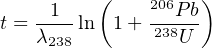
If you want you can use the simplifying approximation that ln(1+X) ≈ X if X ≪ 1 (this assumption may not be correct for the ²⁰⁷Pb/²³⁵U-age).
Compute the analytical uncertainties associated with the linear extrapolation of the argon signals of the sample and the standard in Section 12.4. If you use R, the covariance matrix of the slope and intercept can be simply obtained from the vcov(fit) function, where fit is the output of the lm function (see item 8 of Section 12.1). The corresponding standard errors are then found by taking the square root of the diagonal elements of this matrix.
For Matlab, all the relevant information is provided in the output of the polyfit function:
help(polyfit)
...
[P,S] = POLYFIT(X,Y,N) returns the polynomial
coefficients P and a structure S for use with
POLYVAL to obtain error estimates for predictions.
S contains fields for the triangular factor (R)
from a QR decomposition of the Vandermonde matrix
of X, the degrees of freedom (df), and the norm
of the residuals (normr). If the data Y are
random, an estimate of the covariance matrix
of P is (Rinv*Rinv')*normr^2/df, where Rinv
is the inverse of R.

Based on these instructions, I have written the following function to calculate the standard errors of the fitting parameters from the second output parameter of the polyfit function:
function se = S2se(S)
covmat = (inv(S.R)*inv(S.R'))*S.normr^2/S.df;
se = sqrt(diag(covmat));
end
Use these error estimates to propagate the analytical uncertainty of the J-value and the sample age. Again you can use the linear approximation to the age equation mentioned in point 3.

12.6 Fission tracks

In this exercise, you will use your programming skills to calculate some fission track ages. You are given the following datasets:

DUR.csv: a table with two columns listing the number of spontaneous tracks N_s and induced tracks N_i counted in 25 grains of an apatite age standard (t = 31.4 Ma) from Durango, Mexico. Note that these pairs of tracks were counted over the same area, so that ρ_s∕ρ_i = N_s∕N_i in Equation 7.9.
MD.csv: a similar table for an apatite sample from Mount Dromedary, Australia.

You will need to:

Rewrite Equation 7.9 in terms of the ζ calibration factor and use this new formula to calculate the ζ factor for each single grain analysis of the Durango age standard. Use a dosimeter track density of ρ_D = 300,000 cm^-2.
Use the mean of these ζ factors to calculate the age of the Mount Dromedary sample (i.e., the single grain ages and their mean).
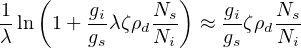
Propagate the analytical uncertainties for each of those single grain ages, using the fact that fission track counts (N, say) follow a Poisson distribution for which it is true that:

$σ2N = N$
To simplify the calculations, you can also use the following approximation:

$1 ( gi Ns ) gi Ns λ-ln 1 + g-λζρdN-- ≈ g-ζρdN-- s i s i$
How does the single grain age precision of the fission track method compare to the U-Pb and ⁴⁰Ar/³⁹Ar age uncertainties in Sections 12.3 and 12.4? Also compare with the standard deviation and standard error of the mean age of Mount Dromedary apatite.

[prev] [prev-tail] [front] [up]

Chapter 12Programming practicals