Structured Illumination and the Optical Transfer Function
The ability of a lens or optical system to pass information -- which as far as
we're concerned here means to form an image -- can be characterised in
spatial terms by its Point Spread Function, or in frequency
terms by its Optical Transfer Function. The PSF tells you the shape of
blurry smudge you'll get in the image plane if you place a single point source
somewhere in the object plane; the OTF tells you the response of the lens to a
given spatial frequency. The OTF is conventionally expressed as the normalised
Fourier transform of the PSF, where normalisation in this case means scaling so
that the value at the zero frequency is 1. The two are to all intents and
purposes equivalent, so which one uses depends on which is more convenient at
the time; often that's the OTF, as in this case.
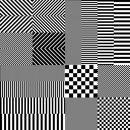
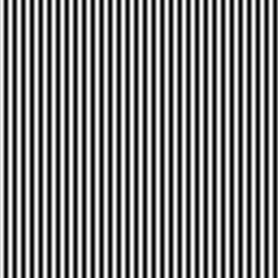
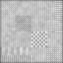
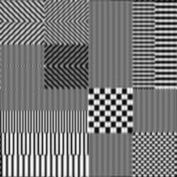
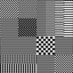
For an idealised circular lens -- ie, one without aberrations -- the OTF is a
fairly simple function of frequency that looks like this:


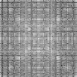


1 But not quite. In fact, the response is proportional to the area of overlap between two copies of the lens pupil separated by an amount representing the frequency; in this case the pupil is circular, which makes the response function simple. At the cut-off frequency and beyond, there is no overlap and thus those frequencies are not transmitted. Alas, this interpretation doesn't hold in the presence of aberrations, which have the effect of distorting the response mapping in unfavourable ways.
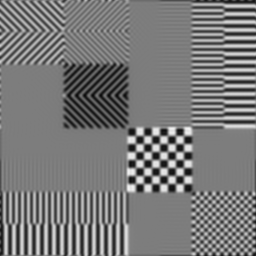
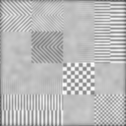
2 This is terribly simplified in this simulation, since we don't model the whole 3d space and consider the degree of defocus, but the general idea should hold true. The actual thickness of the in focus section depends on the frequency of the illumination pattern: the finer the pattern, the tighter the section. Obviously this has to be balanced against the OTF resolution limit, since as the pattern approaches this is becomes more and more indistinct and conveys less and less information.
1 But not quite. In fact, the response is proportional to the area of overlap between two copies of the lens pupil separated by an amount representing the frequency; in this case the pupil is circular, which makes the response function simple. At the cut-off frequency and beyond, there is no overlap and thus those frequencies are not transmitted. Alas, this interpretation doesn't hold in the presence of aberrations, which have the effect of distorting the response mapping in unfavourable ways.
2 This is terribly simplified in this simulation, since we don't model the whole 3d space and consider the degree of defocus, but the general idea should hold true. The actual thickness of the in focus section depends on the frequency of the illumination pattern: the finer the pattern, the tighter the section. Obviously this has to be balanced against the OTF resolution limit, since as the pattern approaches this is becomes more and more indistinct and conveys less and less information.