10 Error propagation

Chapter 10
Error propagation

All the methods and equations presented thus far have assumed that all parameters are either known or measured with infinite precision. In reality, however, the analytical equipment used to measure isotopic compositions, elemental concentrations and radioactive half-lives is not perfect. It is crucially important that we quantify the resulting analytical uncertainty before we can reliably interpret the resulting ages.

For example, suppose that the extinction of the dinosaurs has been dated at 65 Ma in one field location, and a meteorite impact has been dated at 64 Ma elsewhere. These two numbers are effectively meaningless in the absence of an estimate of precision. Taken at face value, the dates imply that the meteorite impact took place 1 million years after the mass extinction, which rules out a causal relationship between the two events. If, however, the analytical uncertainty is significantly greater than 1 Myr (e.g. 64 ± 2 Ma and 65 ± 2 Ma), then such of a causal relationship remains very plausible.

10.1 Some basic definitions

Suppose that our geochronological age (t) is calculated as a function (f) of some measurements (X and Y ):

t = f(X, Y)

(10.1)

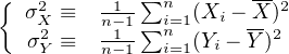
Suppose that we have performed a large number (n) of replicate measurements of X and Y :

{ X = {X1,X2, ⋅⋅⋅,Xi,⋅⋅⋅,Xn } Y = {Y1,Y2,⋅⋅⋅,Yi,⋅⋅⋅,Yn}

(10.2)

It is useful to define the following summary statistics:

The mean:
${ X-≡ 1 ∑n Xi Y-≡ n1 ∑ni=1Yi n i=1$ (10.3)

is a useful definition for the ‘most representative’ value of X and Y , which can be plugged into Equation 10.1 to calculate the ‘most representative’ age.
The variance:
${ σ2 ≡ --1 ∑n (X - X)2 X2 n-11∑ni=1 i -- 2 σY ≡ n- 1 i=1(Yi - Y )$ (10.4)

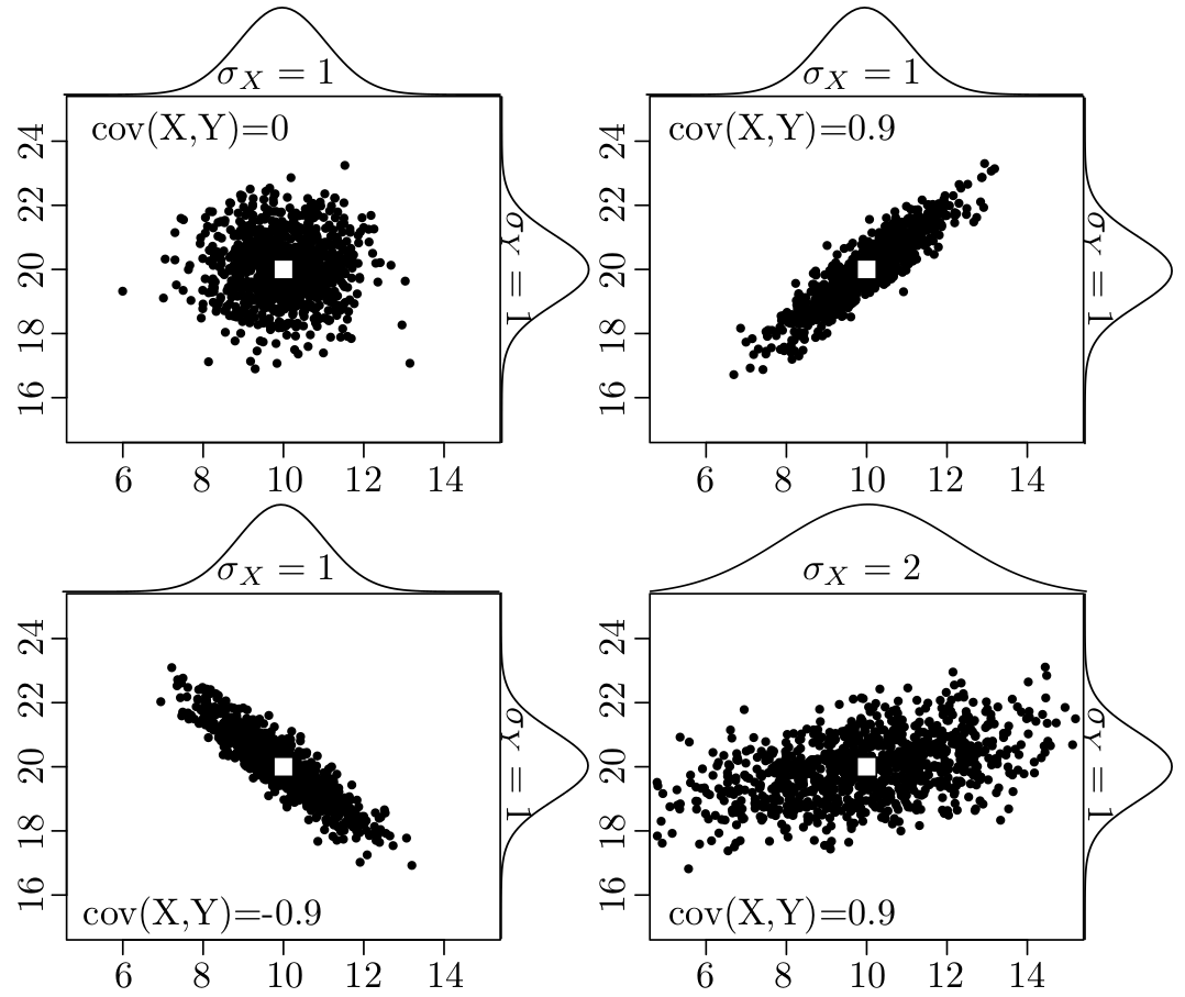
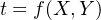
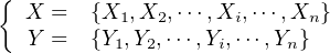
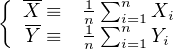
with σ_X and σ_Y the ‘standard deviations’, is used to quantify the amount of dispersion around the mean.
The covariance:
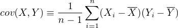$1 ∑n -- -- cov(X,Y ) ≡ n-- 1 (Xi - X )(Yi - Y ) i=1$ (10.5)

quantifies the degree of correlation between variables X and Y .

X, Y , σ_X², σ_Y² and cov(X,Y ) can all be estimated from the input data (X,Y ). These values can then be used to infer σ_t², the variance of the calculated age t, a process that is known as ‘error propagation’. To this end, recall the definition of the variance (Equation 10.4):

1 ∑n - σ2t ≡----- (ti - t)2 n - 1i=1

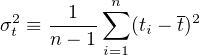(10.6)

We can estimate (t_i -t) by differentiating Equation 10.1:

ti - t = (Xi - X-) ∂f-+ (Yi - Y)-∂f ∂X ∂Y

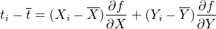(10.7)

Plugging Equation 10.7 into 10.6, we obtain:

σ_t²	= ∑ _i=1ⁿ²	(10.8)
	= σ_X²² + σ_Y²² + 2 cov(X,Y )	(10.9)

This is the general equation for the propagation of uncertainty with two variables, which is most easily extended to more than two variables by reformulating Equation 10.9 into a matrix form:

[ ][ ∂t ] σ2= [ -∂t-∂t-] σ2X cov(X,Y ) ∂X- t ∂X ∂Y cov(X,Y ) σ2Y ∂∂tY-

(10.10)

where the innermost matrix is known as the variance-covariance matrix and the outermost matrix (and its transpose) as the Jacobian matrix. Let us now apply this equation to some simple functions.

10.2 Examples

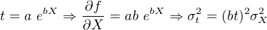
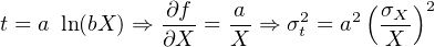
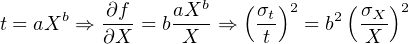
Let X and Y indicate measured quantities associated with analytical uncertainty. And let a and b be some error free parameters.

addition:

t = aX + bY ⇒ = a, = b
⇒ σ_t² = a²σ_X² + b²σ_Y² + 2ab cov(X,Y ) (10.11)
subtraction:
$t = aX - bY ⇒ σ2= a2σ2 + b2σ2 - 2ab cov(X,Y ) t X Y$ (10.12)

multiplication:

	t = aXY ⇒ = aY, = aX
	⇒ σ_t² = (aY )²σ_X² + (aX)²σ_Y² + 2a²XY cov(X,Y )
	⇒² = ² + ² + 2	(10.13)

division:
$X ( σt)2 ( σX)2 (σY )2 cov(X,Y ) t = a-Y ⇒ t- = X-- + Y-- - 2---XY----$ (10.14)
exponentiation:
$∂f t = a ebX ⇒ ---= ab ebX ⇒ σ2t = (bt)2σ2X ∂X$ (10.15)
logarithms:
$∂f a 2 2( σX )2 t = a ln(bX ) ⇒ ∂X = X-⇒ σt = a X--$ (10.16)
power:
$∂f aXb ( σt)2 ( σX)2 t = aXb ⇒ ∂X- = b-X--⇒ t- = b2 X--$ (10.17)

10.3 Accuracy vs. precision

Recall the definition of the arithmetic mean (Equation 10.3):

n X- ≡ 1∑ X n i=1 i

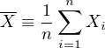
Applying the equation for the error propagation of a sum (Equation 10.11):

1 ∑n σ2 σ2X-= -- σ2Xi = -X- n i=1 n

(10.18)

where we assume that all n measurements were done independently, so that cov(X_i,X_j) = 0∀i,j. The standard deviation of the mean is known as the standard error:

σ σX-= √X-- n

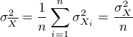
(10.19)

This means that the standard error of the mean monotonically decreases with the square root of sample size. In other words, we can arbitrarily increase the precision of our analytical data by acquiring more data. However, it is important to note that the same is generally not the case for the accuracy of those data. The difference between precision and accuracy is best explained by a darts board analogy:

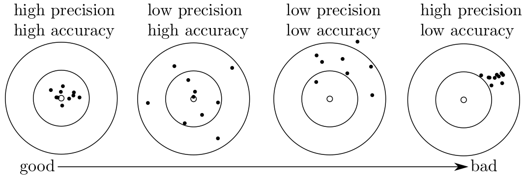
Whereas the analytical precision can be computed from the data using the error propagation formulas introduced above, the only way to get a grip on the accuracy is by analysing another sample of independently determined age. Such test samples are also known as ‘secondary standards’.

Figure 10.1: Four datasets of 100 random numbers (black dots) which have the same means (white squares) but different (co-)variance structures. The marginal distributions of the X and Y variables are shown as ‘bell curves’ on the top and right axis of each plot.

[next] [prev] [prev-tail] [front] [up]

	t = aX + bY ⇒ = a, = b
	⇒ σ_t² = a²σ_X² + b²σ_Y² + 2ab cov(X,Y )	(10.11)

Chapter 10Error propagation

10.1 Some basic definitions

10.2 Examples

10.3 Accuracy vs. precision

Chapter 10
Error propagation