Fresa dynamic optimization tutorial
Table of Contents
| Author | Professor Eric S Fraga (e.fraga@ucl.ac.uk) |
| Last revision | 2023-06-02 13:06:44 |
Introduction
The Fresa and Strawberry packages provide general single and multi-objective optimization procedures for black-box models.

Black box models do not provide gradient information. They may also be computationally expensive and so estimating gradients numerically may be computationally intractable. These models may also be discontinuous and so gradients may be undefined. For such problems, direct search and stochastic methods may be more appropriate.
The Fresa and Strawberry methods implement a Plant Propagation Algorithm. This is a stochastic population based evolutionary approach which mimics the behaviour of strawberry plants in their search for good locations to set down roots. Both methods support both single and multi-objective problems. Fresa is written in the Julia language while Strawberry is written in the Octave language (which is mostly compatible with MATLAB).
This document presents a simple tutorial, using Fresa, which illustrates the implementation of a differential equation based model, the associated optimization based design problem, and how the latter can be solved. A multi-objective version of the design problem is considered.
The problem
The design problem is an adaptation of the batch reactor problem described by Cizniar et al.1. Given the reaction
![\[ \ce{A -> B -> C} \]](ltximg/tutorial_1c330277fbd47f1db8fa68611a1f3bd0f73b0cf9.png)
the original problem was to determine the temperature profile which leads to the best yield of a desired product, B, in a batch reactor. We have modified the problem to also consider minimizing the concentration of the undesired product, C. We shall see, below, that adding this second objective for the design problem can lead to better understanding the trade-off between different solutions that would be missed using a single objective optimization approach.
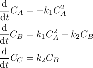
The reactions are modelled mathematically as follows:
with

with ![\(t \in [0,1]\)](ltximg/tutorial_5c9f03c2269750951ce07f86833141bb9926934e.png) and
and  to be determined for optimum operation.
The remainder of this section presents the Julia code for defining the design problem and using Fresa to find the set of non-dominated solutions for the two criteria specified. The full code is available at gitlab as BatchReactor.jl. To use this code in Julia,
$ julia
]
add Fresa
add https://gitlab.com/ericsfraga/BatchReactor.jl
BACKSPACE
C-d
where ] enters the package manager in Julia, BACKSPACE returns to the normal REPL, and C-d (control key with d) exits Julia.
Start of code
The recommended approach in Julia is to have all related functions in a module. We will create a BatchReactor module and the majority of the code in this tutorial will reside in this module. There will be other files associated with this that illustrate how the module is used to solve the design problem and present results.
module BatchReactor

using DifferentialEquations     # for solving the system of ODEs
using Fresa                     # for optimization
using Printf                    # for formatted output
using PyPlot                    # for plotting profiles
Temperature profile
The decision variable for the optimization problem is the temperature profile. This is a continuous quantity over time. There are many ways this variable could be implemented. The temperature profile will be manipulated by the optimization method (i.e. Fresa). In this section, we define two alternative representations of temperature profiles to highlight the flexibility of Fresa and the power of the Julia language for describing and manipulating data structures.
The specific batch reactor design problem requires a time interval, [0,tfinal], and that the temperature be bounded:
const tfinal = 1.0              # no units given in paper
const Tmin = 298.0              # Kelvin
const Tmax = 398.0              # Kelvin
As we wish to consider different representations for temperature profiles so we create a base, abstract, type which the others implement.
abstract type TemperatureProfile end
Adaptive piece-wise linear profile
The simplest profile representation is a vector of values corresponding to a piece-wise linear function of the temperature for a uniformly distributed set of time intervals. However, this can be inefficient as the number of intervals may need to be large to ensure that the spacing is small enough where needed. Instead, we wish to use an adaptive discretization of the time interval and allow the optimization procedure to actually choose the size of each interval. This is similar to the first approach used by Rodman et al. (2018).2
The profile definition
The temperature profile is defined by a set of nt tuples, (Δti, ΔTi), i=1,…,nt, each of which defines the size of the i-th interval and the change in temperature over that interval, assuming a linear change. The Δ values are given as a fraction of the maximum values allowed. The i-th tuple is (ft,fT) where ft ∈ [0,1] and fT ∈ [-1,1]. The temperature can go both up and down at any time. The size of the i-th interval is ft × (tf - ti-1) where tf is the final time. For the temperature, we will have a maximum change allowed, ΔTmax, and the new temperature at the end of time interval i will be Ti-1 + fT × ΔTmax.
t0 is 0 and T0, the initial temperature in the reactor, is a decision variable. The total number of variables which the optimization procedure can manipulate is therefore 2 × nt + 1. The number of intervals to have must be specified a priori and we will see later how this is defined implicitly.
The actual definition of the decision variables is embodied in a data structure and consists of two vectors of values, one for the ft values and one for fT, and the initial temperature, T0. The use of a custom type allows us to have error checking built-in and will also aid in the presentation of results and in customization of the evolutionary search used by Fresa.
mutable struct PiecewiseLinearProfile <: TemperatureProfile
    ft :: Array{Float64}        # time deltas
    fT :: Array{Float64}        # temperature deltas
    T0 :: Float64               # initial temperature
    function PiecewiseLinearProfile(ft, fT, T0)
        if length(ft) != length(fT)
            error("Number of time points and temperature changes must match.")
        end
        if T0 < Tmin || T0 > Tmax
            error("T0 = $(T0) not in [$Tmin,$Tmax]")
        end
        new(ft,fT,T0)
    end
    function PiecewiseLinearProfile(t :: PiecewiseLinearProfile)
        new(t.ft, t.fT, t.T0)
    end
end
# allow up to 10 degrees change per time interval
ΔT_max = 10.0
The temperature as function of time
The temperature profile is used within the simulation code to determine the temperature for any time . If the desired time is past the final time defined by the vector, the last temperature value will be used; in other words, we assume a constant temperature past the end of the profile defined by the tuple vector until the final time.
function temperature(profile :: PiecewiseLinearProfile, t :: Float64) :: Float64
    τ = 0
    T = profile.T0
    for i=1:length(profile.ft)
        Δτ = profile.ft[i] * (tfinal - τ)
        ΔT = profile.fT[i] * ΔT_max
        if t < τ + Δτ
            # partial step to reach desired time
            T += ΔT * (t-τ)/Δτ
            # correct T if out of bounds
            if T < Tmin
                T = Tmin
            elseif T>Tmax
                T = Tmax
            end
            # leave loop
            break
        else
            # take full step
            T += ΔT
            # correct T if out of bounds
            if T < Tmin
                T = Tmin
            elseif T>Tmax
                T = Tmax
            end
        end
        τ += Δτ
    end
    return T
end
Formatted output of temperature profile
Although Julia will output the contents of any user defined type in a mostly readable fashion, it is often convenient to provide an output method for the type. This following code segment does just that for the PiecewiseLinearProfile type:
function Base.show(io::IO, profile::BatchReactor.PiecewiseLinearProfile)
    @printf(io, "PWL | %.4g ", profile.T0)
    for i = 1:length(profile.ft)
        @printf(io, "| %.4g ", profile.ft[i])
    end
    for i = 1:length(profile.fT)
        @printf(io, "| %.4g ", profile.fT[i])
    end
end
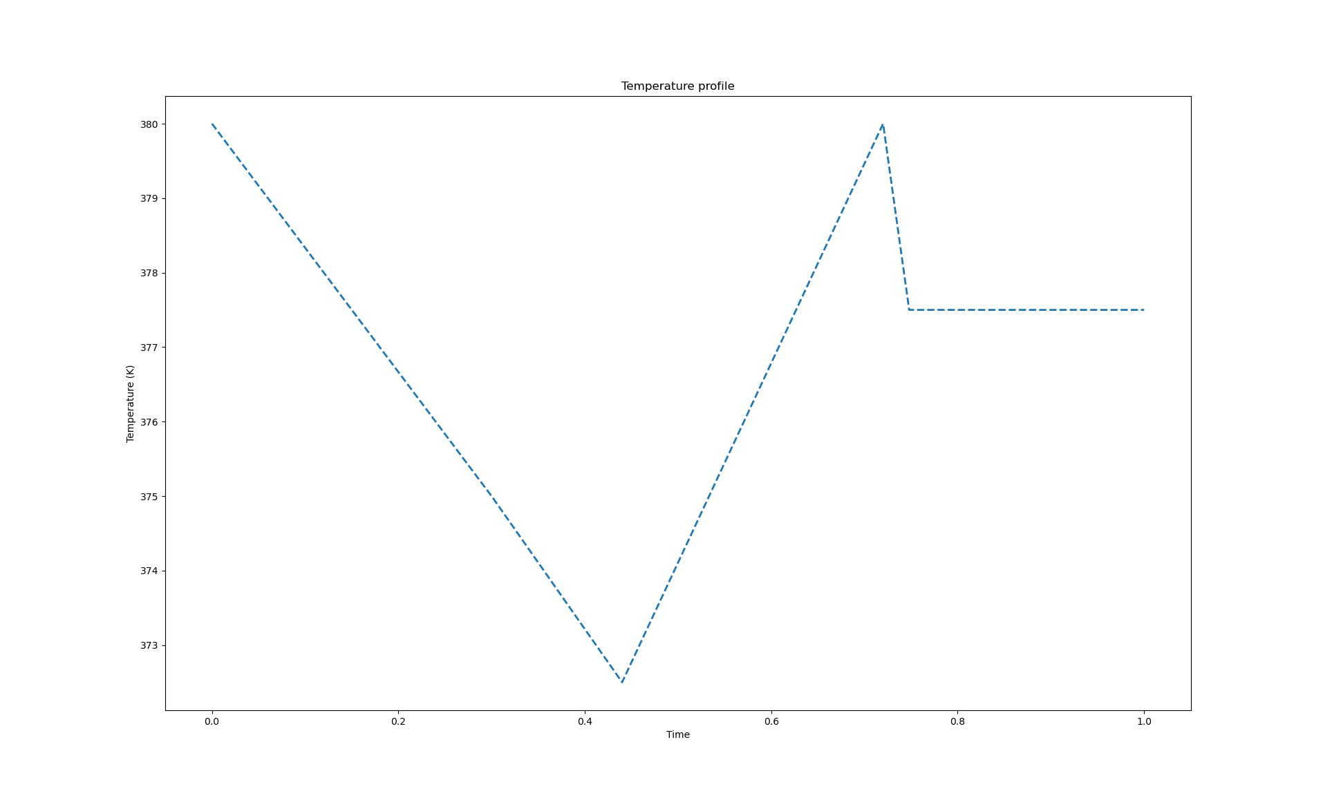
Example profile
The following code will generate a temperature profile shown in the figure below. Although this is probably not a desired temperature profile, it illustrates the types of profiles that can be represented.
using BatchReactor
using PyPlot
profile = BatchReactor.PiecewiseLinearProfile([0.3; 0.2; 0.5; 0.1],
                                              [-0.5; -0.25; 0.75; -0.25],
                                              380.0)
BatchReactor.plot(profile)
PyPlot.savefig("piecewiselinearprofile.png")
Quadratic spline profile
In some cases, we would prefer to have a particular shape or a shape with specific properties. For instance, we may wish to have a temperature profile that moves away from the initial temperature gradually initially and also comes to a final temperature in a smooth gradual fashion. The following profile is based on splitting the time domain in two, at 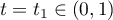 , and fitting a quadratic to each half of the domain. The two quadratics will have 0 slope at the bounds of the overall time domain and equal slope at the point where they meet.
The use of this profile will restrict the search to temperature profiles that are smooth but monotonic in behaviour: either increasing or decreasing temperature throughout the interval. Should this not be what was a desired, higher order polynomials, or in fact any other function, could be used. See the previously cited article by Rodman et al., 2018, for how a temperature profile was represented using 4th and 5th order polynomials with three sub-intervals.
maxima code for quadratic splines
Use Maxima to find the coefficients of two quadratics that meet the requirements specified, given values for T0, the initial temperature, t1, the time point at which the two quadratics meet, and Tf, the final temperature.
T1(t) := a + b*t + c*t^2;
define(dT1(t), diff(T1(t),t));
T2(t) := d + e*t + f*t^2;
define(dT2(t), diff(T2(t),t));
equations: [T1(0) = T0,
dT1(0) = 0,
dT1(t1) = dT2(t1),
dT2(1.0) = 0.0,
T1(t1) = T2(t1),
T2(1.0)=Tf];
solution: solve(equations, [a,b,c,d,e,f]);
for i: 1 thru length(solution[1]) do print(solution[1][i])$
a = T0
b = 0
      T0 - Tf
c = - -------
        t1
      T0 - Tf t1
d = - ----------
        t1 - 1
    2 T0 - 2 Tf
e = -----------
      t1 - 1
      T0 - Tf
f = - -------
      t1 - 1
The profile
mutable struct QuadraticSplineProfile <: TemperatureProfile
    T0 :: Float64               # initial temperature
    Tf :: Float64               # final temperature
    t1 :: Float64               # time point
    a :: Float64                # coefficients of quadratics
    b :: Float64
    c :: Float64
    d :: Float64
    e :: Float64
    f :: Float64
    function QuadraticSplineProfile(T0, Tf, t1)
        a = T0
        b = 0
        c = (Tf-T0)/t1
        d = (Tf*t1 - T0) / (t1 - 1)
        e = (2*T0 - 2*Tf) / (t1 - 1)
        f = (Tf - T0) / (t1 - 1)
        new(T0, Tf, t1, a, b, c, d, e, f)
    end
end
Temperature from profile
The method to determine the temperature for any time t is much easier for this temperature profile: we have two sub-intervals and a quadratic for each sub-interval that describes the behaviour of the temperature. We simply have to evaluate the appropriate quadratic.
function temperature(p :: QuadraticSplineProfile, t :: Float64) :: Float64
    if t <= p.t1
        T = p.a + p.b*t + p.c*t^2
    else
        T = p.d + p.e*t + p.f*t^2
    end
    return T
end
Formatted output
As the quadratic spline profile structure has a number of extra fields (coefficients a through f) and as these are not of interest in general, we override the show function to provide a custom representation of instances of this structure:
function Base.show(io :: IO, profile :: BatchReactor.QuadraticSplineProfile)
    @printf(io, "QSP | %.3g | %.3g | %6.5g ", profile.T0, profile.Tf, profile.t1)
end
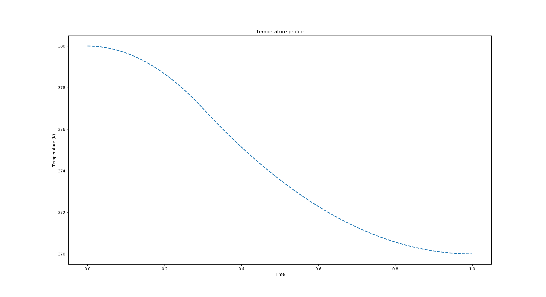
Example profile
The following code will generate a quadratic spline profile with plot shown below. This is a much smoother profile than the example shown for the piecewise linear profile example earlier.
using BatchReactor
using PyPlot
profile = BatchReactor.QuadraticSplineProfile( 380.0, 370.0, 0.3 )
BatchReactor.plot(profile)
PyPlot.savefig("quadraticsplineprofile.png")
Plot a profile
Little function to plot out a quadratic spline profile. This has been used to illustrate the temperature profiles above.
function plot( profile :: TemperatureProfile )
    n = 1000
    δx = 1.0/1000
    x = [(i-1)*δx for i in 1:n+1]
    y = [temperature(profile,x[i]) for i in 1:n+1]

    PyPlot.plot(x,y, linewidth=2.0, linestyle="--", )
    PyPlot.ylabel("Temperature (K)")
    PyPlot.xlabel("Time")
    PyPlot.title("Temperature profile")
end
The reaction
The reaction taking place in the batch reactor is modelled using a set of ordinary differential equations. The A → B reaction is second order reaction and B → C is first order. The model consists of three differential equations, one for each species and depends on the rate constants, k, which are a function of the temperature. The code which implements this model expects a parameter, p, which is the temperature profile. We state that this parameter is of type TemperatureProfile, the abstract type we defined above. This ensures that the parameter actually passed to this method will be an instance of one of the temperature profile types also defined above.
function reactor(x :: Array{Float64,1},
                 p :: TemperatureProfile,
                 t :: Float64
                 ) :: Array{Float64,1}
    T = temperature(p,t)
    k = rates(T)
    # println("$t $T $k")
    return [-k[1] * x[1]^2
            k[1] * x[1]^2 - k[2] * x[2]
            k[2] * x[2]]
end
The temperature is itself a function of time and is determined using the profile and the associated methods defined earlier specific to each type of profile. The Multiple dispatch capabilities of Julia make this easy to do. The temperature profile will be our decision variable for design and is implemented above. The rate constants are defined below.
Initial concentrations
The system of differential equations along with the initial values for the concentrations define an initial value problem. The initial concentration of A is 1 and there are no B & C present.
x0 = [1.0, 0.0, 0.0]
Reaction rate constants
The rate constants are given by
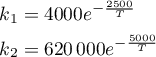
where T ∈ [298,398] K.
rates = T -> [4000.0 * exp(-2500.0/T)
              620000 * exp(-5000.0/T)]
Simulation
Using the model defined above, we can now solve it using an ODE solver to simulate the behaviour over the desired time interval, t ∈ [0,1]. The temperature profile is the argument given to this method and is a TemperatureProfile (see above). The Initial concentration in the reactor is pure A and no B or C, as defined in the x0 variable. The system of differential equations is solved using the DifferentialEquations Julia package.
The result of the simulation method is a data structure consisting of the vector of time points and an array of vectors, where each vector is the set of concentrations of the individual species at the corresponding time point. The number of time points depends on the numerical method used in solving the differential equations and this will vary depending on the temperature profile as the method is likely to be adaptive.
function simulation(profile :: TemperatureProfile)
    # for testing some performance aspects, we have two ways of
    # simulating the reactor, i.e. solving the differential equations:
    # an efficient solver (RK 2-3) and a computationally inefficient
    # one, Euler's method
    efficient = true
    if efficient
        # efficient solver
        tspan = (0.0,tfinal)
        prob = ODEProblem(reactor, x0, tspan, profile)
        results = DifferentialEquations.solve(prob)
        results[end]
    else
        δt = tfinal/1e4
        t = 0.0
        x = x0
        while t < tfinal
            if t+δt > tfinal
                δt = tfinal - t
            end
            δx = δt * reactor(x, profile, t)
            t = t + δt
            x = x + δx
        end
        x                       # end values
    end
end
Optimization
The optimization problem is to maximize the concentration of the second species, B, varying the temperature of the reactor dynamically. We have extended the original problem to include the objective of minimizing the production of the third species, C. The only constraint in the original problem definition is that T be ∈ [298,398] K. We use the Fresa method to find the optimum temperature profile. To do so, we will use the dynamic temperature profile and function defined above with the simulation method.
The objective function
The objective function evaluates the system of differential equations for the given temperature profile, argument profile, and returns the values of the two objectives and the feasibility measure. The first objective is the concentration of the second species, B, multiplied by negative 1, because Fresa assumes that the optimization objective is to minimize and we wish to maximize the concentration. The second objective is the concentration of the 3rd, undesired, species C which we wish to minimize. The indication of feasibility should be less than or equal to 0 when feasible and a value greater than 0 when infeasible. As constructed, all possible temperature profiles lead to feasible designs so the measure of infeasibility we return is always 0.
function objective(profile :: TemperatureProfile)
    results = simulation(profile)
    # take the last concentration of species B, times -1, as the first
    # objective function value and the last concentration of C as the
    # second objective function values.  Also indicate that the design
    # is always feasible.
    ([-results[2], results[3]], 0.0)
end
Solve using Fresa
For many optimization problems, those where the decision variables can be defined by an array of real values, Fresa will require only a starting guess and the objective function. However, if the decision variables have been implemented in a user defined type, Fresa expects one more item: the definition of a neighbouring solution in the design space.
The neighbour function
The neighbour function has 4 arguments: a point in the design space, the lower and upper bounds for decision variables, and a fitness value indicating how good the current point is (in some relative sense based on the population of points at the current point in the evolutionary process). Good points should define neighbours which are close by generally and less good points should define neighbours which are further away. See the description of the neighbour function for the Strawberry method for a longer description.
- Piecewise linear profile
Fresa comes with some pre-defined neighbour functions, specifically for single floating point numbers and vectors of floating point numbers. For the piecewise linear profile, we need to find neighbouring values for each of the two arrays (time points and temperature changes) as well as the initial temperature. We define the function as belonging to Fresa so that the multi-dispatch feature of Julia will find this method automatically according to the arguments passed to the
neighbourfunction.function Fresa.neighbour(x :: PiecewiseLinearProfile, f, domain) a = domain.lower(x) b = domain.upper(x) ft = Fresa.neighbour(x.ft, f, Fresa.Domain(x->a.ft, x->b.ft)) fT = Fresa.neighbour(x.fT, f, Fresa.Domain(x->a.fT, x->b.fT)) T0 = Fresa.neighbour(x.T0, f, Fresa.Domain(x->a.T0, x->b.T0)) PiecewiseLinearProfile(ft,fT,T0) endThis function uses the existing definition of the
neighbourfunction for single floating point numbers.- Quadratic spline profile
For the quadratic spline, the neighbouring solutions will be based on different initial and final temperatures and the time point within the time domain.
function Fresa.neighbour(x :: QuadraticSplineProfile, f, domain)
    a = domain.lower(x)
    b = domain.upper(x)
    T0 = Fresa.neighbour(x.T0, f, Fresa.Domain(x->a.T0, x->b.T0))
    Tf = Fresa.neighbour(x.Tf, f, Fresa.Domain(x->a.Tf, x->b.Tf))
    t1 = Fresa.neighbour(x.t1, f, Fresa.Domain(x->a.t1, x->b.t1))
    QuadraticSplineProfile(T0, Tf, t1)
end
Solve the problem
To use Fresa, we have to provide the objective function, an initial population consisting of points in the design space, and the domain for the search, i.e. lower and upper bounds for the decision variables. Optionally, we can specify a number of arguments which tailor the behaviour of Fresa for the problem at hand. These include the ranking mechanism used for multi-objective optimization problems and the neighbour function for decision variables using user-defined types. For this problem, the neighbour function has to be specified. The other optional arguments can be changed and it is useful to explore the impact of, for instance, the population size on the quality of solutions obtained. The values currently defined work well for this problem.
function solve(p0, domain :: Fresa.Domain)
    Fresa.solve(
        # the first 4 arguments are required
        objective,               # the objective function
        p0;                      # an initial point in the design space
        # the rest are option arguments for Fresa
        domain = domain,         # search domain for the decision variables
        archiveelite = false,    # save thinned out elite members
        elite = true,            # elitism by default
        ϵ = 0.001,               # tolerance for similarity detection
        fitnesstype = :hadamard, # how to rank solutions in multi-objective case
        #fitnesstype = :borda,   # how to rank solutions in multi-objective case
        multithreading = true,   # use multiple threads, if available
        ngen = 100,              # number of generations
        np = 20,                 # population size
        nrmax = 5,               # number of runners maximum
        ns = 100,                # number of stable solutions for stopping
        output = 1)              # how often to output information
end
Random search
The following code is not used in this tutorial but is provided for experimenting with random search methods (not fitness based). Fresa has methods for generating a random population.
function Fresa.randompoint(a :: PiecewiseLinearProfile, b :: PiecewiseLinearProfile)
    PiecewiseLinearProfile(Fresa.randompoint(a.ft, b.ft),
                           Fresa.randompoint(a.fT, b.fT),
                           Fresa.randompoint(a.T0, b.T0))
end
function Fresa.randompoint(a :: QuadraticSplineProfile, b :: QuadraticSplineProfile)
    QuadraticSplineProfile(Fresa.randompoint(a.T0, b.T0),
                           Fresa.randompoint(a.Tf, b.Tf),
                           Fresa.randompoint(a.t1, b.t1))
end
End of code
All the code presented in the sections above are withing the BatchReactor module. We need to finish off the module before we can start using it.
end
Running the model
Simulation test
We can use the simulation method directly to explore different temperature profiles manually. I used this to test out the encoding and decoding of temperature profiles.
PiecewiseLinearProfile simulation test
This code can be found in the gitlab repository for the tutorial (https://gitlab.com/ericsfraga/BatchReactor.jl) as test/testsimulation.jl which you can download. You would then run it by executing the following command at the terminal window or REPL (e.g. within Emacs):
julia testsimulation.jl
using BatchReactor
# define a temperature profile
profile = BatchReactor.PiecewiseLinearProfile(
    [0.5 1.0],  # half the time in first interval
    [0.0 -0.5], # constant first interval, down by half amount allowed in second
    398.0)      # use the maximum temperature allowed as initial temperature
# simulate the process
results = BatchReactor.simulation(profile)
println("Results from simulation: $results")
# # plot out the results, i.e. the concentrations of all species as a
# # function of time.
# using PyPlot
# PyPlot.plot(results.t, [results.u[i][1] for i=1:length(results.u)])
# PyPlot.plot(results.t, [results.u[i][2] for i=1:length(results.u)])
# PyPlot.plot(results.t, [results.u[i][3] for i=1:length(results.u)])
# PyPlot.xlabel("t")
# PyPlot.ylabel("Concentration")
# PyPlot.savefig("testsimulation.pdf")
The concentration profiles from the simulation are plotted out. This uses the PyPlot package which will need to be installed if it hasn't been already. Use Pkg.install("PyPlot") to do this in Julia.
QuadraticSplineProfile simulation test
This code can be found in the gitlab repository for the tutorial (https://gitlab.com/ericsfraga/BatchReactor.jl) as test/testsimulationquadratic.jl which you can download. You would then run it by executing the following command at the terminal window or REPL (e.g. within Emacs):
julia testsimulationquadratic.jl
using BatchReactor
profile = BatchReactor.QuadraticSplineProfile(350.0, 290.0, 0.5)
results = BatchReactor.simulation(profile)
using PyPlot
PyPlot.plot(results.t, [results.u[i][1] for i=1:length(results.u)])
PyPlot.plot(results.t, [results.u[i][2] for i=1:length(results.u)])
PyPlot.plot(results.t, [results.u[i][3] for i=1:length(results.u)])
PyPlot.xlabel("t")
PyPlot.ylabel("Concentration")
PyPlot.savefig("testsimulationquadratic.pdf")
Optimization tests
To solve the problem, all we have to do is invoke the solve method in the BatchReactor module, giving an initial solution. The solve method returns the set of non-dominated solutions in the final population along with that final population. A non-dominated solution is one that is better than all other solutions for at least one of the criteria.
The following codes calls the solve method with different initial profiles.
Piecewise linear example
The code for this example can be found in the gitlab repository for the tutorial (https://gitlab.com/ericsfraga/BatchReactor.jl) as test/pwltestoptimization.jl which you can download. You would then run it by executing the following command at the terminal window or REPL (e.g. within Emacs):
julia pwltestoptimization.jl
using BatchReactor
using Fresa
# bounds
domain = Fresa.Domain(x -> BatchReactor.PiecewiseLinearProfile(zeros(length(x.ft)),
                                                               -ones(length(x.fT)),
                                                               BatchReactor.Tmin),
                      x -> BatchReactor.PiecewiseLinearProfile(ones(length(x.ft)),
                                                               ones(length(x.fT)),
                                                               BatchReactor.Tmax))
# create initial population consisting of just the initial profile
p0 = [Fresa.Point(BatchReactor.PiecewiseLinearProfile([0.5, 0.5, 0.5, 0.5], [0.0, 0.0, 0.0, 0.0], 323.0),
                  BatchReactor.objective)]
# invoke Fresa
nondominated, population = BatchReactor.solve(p0, domain)
println("Non-dominated solutions:")
println("$(population[nondominated])")
println("Full population:")
println("$population")
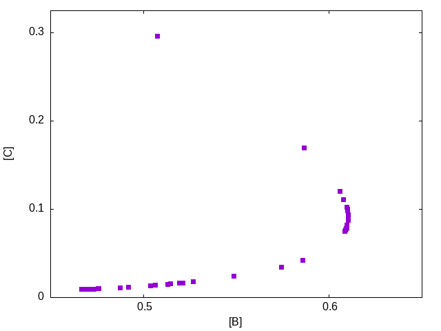
The following figure shows the final population, plotting one objective function ([C]) as a function of the other ([B]) showing the trade-off between the two. The non-dominated points are those along the bottom up to the right-most point in the plot. Recall that we wish to maximize the concentration of B, [B], while minimizing the concentration of C, [C].
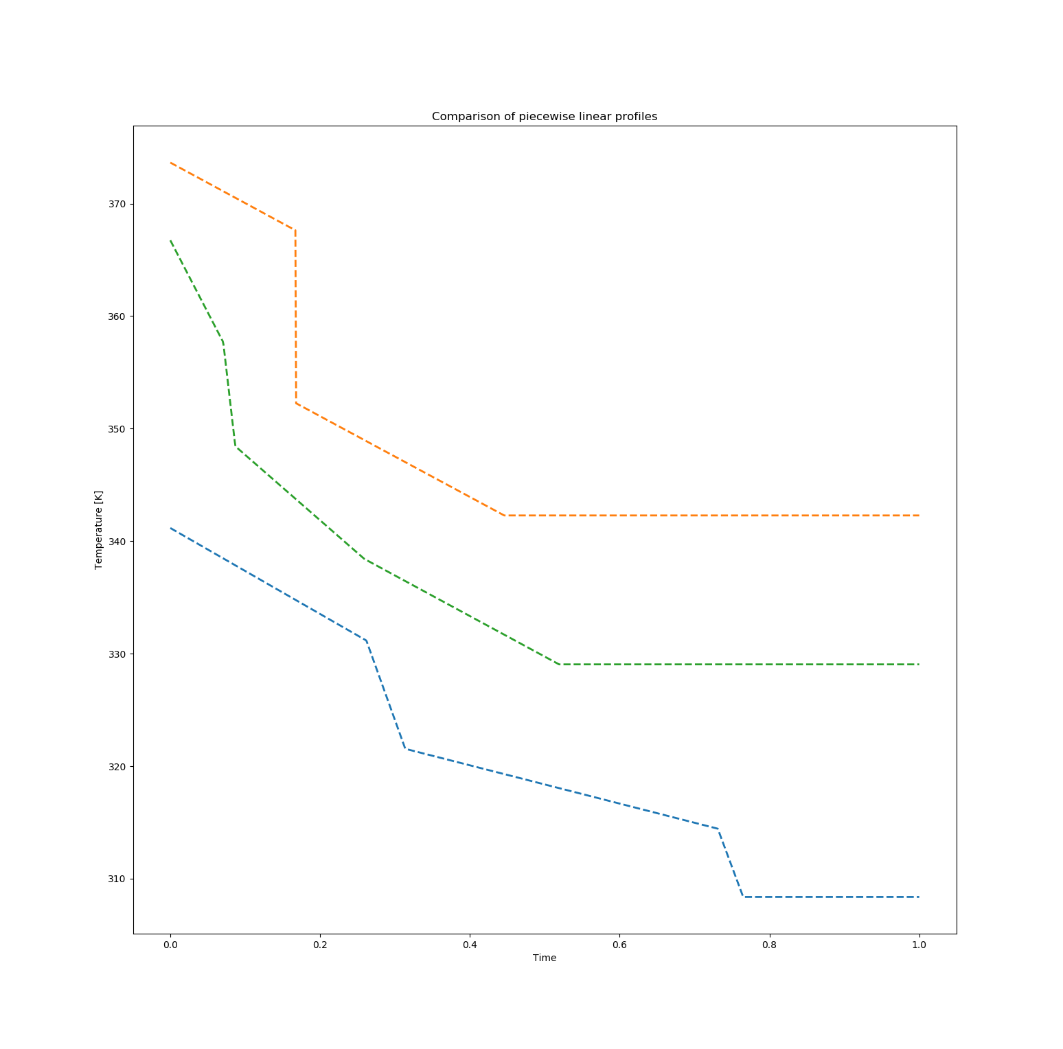
The following plots presents the best solution for maximizing [B], the middle profile, along with two solutions with concentration of B of approximately 0.58 but with significantly different values for the final concentration of C, specifically with values of 0.042 (bottom profile) and 0.170 (top profile). The profiles for these two solutions are shown in Figure figure-pwlcomparison.
Quadratic spline example
Using the quadratic spline representation (file test/qsptestoptimization.jl in the gitlab repository),
using BatchReactor
using Fresa
# bounds
domain = Fresa.Domain(x -> BatchReactor.QuadraticSplineProfile(BatchReactor.Tmin, BatchReactor.Tmin, 0.25),
                      x -> BatchReactor.QuadraticSplineProfile(BatchReactor.Tmax, BatchReactor.Tmax, 0.75))
# create initial population consisting of just the initial profile
p0 = [Fresa.Point(BatchReactor.QuadraticSplineProfile(323.0, 323.0, 0.5),
                  BatchReactor.objective)]
# invoke Fresa
nondominated, population = BatchReactor.solve(p0, domain)
println("Non-dominated solutions:")
println("$(population[nondominated])")
println("Full population:")
println("$population")
The outcome, in terms of objective function values, is similar:
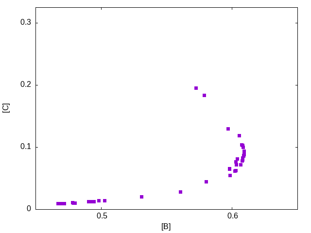
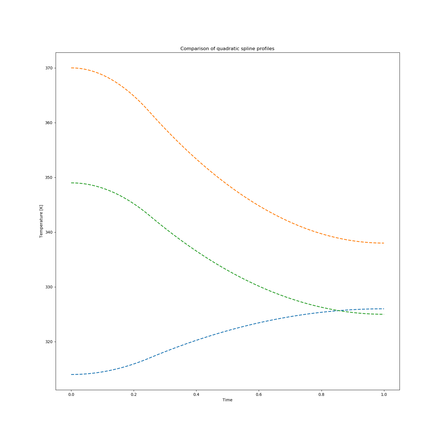
and we can again compare some solutions from this population. In the following figure, the middle profile is the best solution in terms of the concentration of B achieved. The other two solutions correspond to concentrations of B of approximately 0.58 with the top one achieving a concentration of C of 0.20 and the bottom one achieving [C]=0.044.
Both at the same time
One of the features of Fresa is the generic nature of the implementation, allowing for different representations and also values of the objective function. The latter is not illustrated in this tutorial (please contact the author if this might be of interest). The former has been illustrated through the definition of two different representations of temperature profiles.
However, we can take this one step further: we can pass a population of initial solutions to Fresa and this population can include solutions with different representations. Fresa does not use any form of recombination of solutions in the propagation for the creation of new solutions. Therefore, the population can comfortably consist of different representations. We illustrate this by providing a population consisting of a single piecewise linear profile and a single quadratic spline profile. The code is found in test/genericoptimization.jl in the gitlab repository.
The only complexity introduced by having multiple representations in a population is that the lower and upper bounds of the domain have to be defined to return appropriate results for different representations. The code below shows the use of the typeof function in Julia to cater for the different temperature profile representations.
using BatchReactor
using Fresa
# bounds
function lower(p :: BatchReactor.TemperatureProfile)
    if typeof(p) == BatchReactor.PiecewiseLinearProfile
        BatchReactor.PiecewiseLinearProfile(zeros(length(p.ft)),-ones(length(p.fT)),BatchReactor.Tmin)
    else
        BatchReactor.QuadraticSplineProfile(BatchReactor.Tmin, BatchReactor.Tmin, 0.25)
    end
end
function upper(p :: BatchReactor.TemperatureProfile)
    if typeof(p) == BatchReactor.PiecewiseLinearProfile
        BatchReactor.PiecewiseLinearProfile(ones(length(p.ft)),ones(length(p.fT)),BatchReactor.Tmax)
    else
        BatchReactor.QuadraticSplineProfile(BatchReactor.Tmax, BatchReactor.Tmax, 0.75)
    end
end
domain = Fresa.Domain(lower, upper)
# create initial population consisting of one initial profile for each type of representation
p0 = [Fresa.Point(BatchReactor.QuadraticSplineProfile(323.0, 323.0, 0.5), BatchReactor.objective)
      Fresa.Point(BatchReactor.PiecewiseLinearProfile([0.5, 0.5, 0.5, 0.5], [0.0, 0.0, 0.0, 0.0], 323.0),
                  BatchReactor.objective)]
# invoke Fresa
nondominated, population = BatchReactor.solve(p0, domain)
println("Non-dominated solutions:")
println("$(population[nondominated])")
println("Full population:")
println("$population")
Recent change history
2023-06-02 updated tutorial for version 8 of Fresa
2023-06-02 random point method added for analysis of performance
2021-12-03 fix versioning, adding tag to master
2021-12-03 added a method for exploring the space randomly
2021-06-04 fixed missing Δ in description of quadratic spline profile
2021-06-02 added mathematical description of reaction model
2021-05-26 Minor change to order of 'using' statements to remove clutter
2021-05-26 played around with multithreading in Fresa
2021-04-23 remove spurious output line and cache black box model image creation
2021-04-23 Implement example with multiple simultaneous representations
Footnotes:
Example 6: DYNOPT User's Guide version 4.1.0, Batch reactor with reactions: A -> B -> C. M. Cizniar, M. Fikar, M. A. Latifi, MATLAB Dynamic Optimisation Code DYNOPT. User's Guide, Technical Report, KIRP FCHPT STU Bratislava, Slovak Republic, 2006.
A Rodman, E S Fraga, D Gerogiorgis (2018), On the application of a nature-inspired stochastic evolutionary algorithm to constrained multiobjective beer fermentation optimisation, Computers & Chemical Engineering 108:448–459, doi:10.1016/j.compchemeng.2017.10.019.