- Introduction
- 1. Introduction to Quantitative Analysis
- 2. Descriptive Statistics
- 3. T-test for Difference in Means and Hypothesis Testing
- 4. Bivariate linear regression models
- 5. Multiple linear regression models
- 6. Assumptions and Violations of Assumptions
- 7. Interactions
- 8. Panel Data, Time-Series Cross-Section Models
- 9. Binary models: Logit
- 10. Frequently Asked Questions
- 11. Optional Material
- 12. Datasets
- 13. R Resources
- 14. References
- Published with GitBook
7. Interactions
7.2 Solutions
Exercise 1
Using our model z.out , where we included the square of GDP/capita, what is the effect of:
- an increase of GDP/captia from $5,000 to $15,000?
- an increase of GDP/capita from $25,000 to $35,000?
Solution
Load the necessary packages
library(foreign)
library(texreg)
library(Zelig)
library(dplyr)
Clear the workspace
rm(list = ls())
Load the dataset and rename the variables to something sensible
qog_data <- read.dta("QoG2012.dta")

qog_data <- rename(qog_data,
                   hdi = undp_hdi,
                   gdp = wdi_gdpc)
We will re-estimate the same model we had done in class.
z.out <- zelig(hdi ~ gdp + I(gdp^2), model = "ls", data = qog_data)
How to cite this model in Zelig:
  R Core Team. 2007.
  ls: Least Squares Regression for Continuous Dependent Variables
  in Christine Choirat, James Honaker, Kosuke Imai, Gary King, and Olivia Lau,
  "Zelig: Everyone's Statistical Software," http://zeligproject.org/
summary(z.out)
Model:

Call:
z5$zelig(formula = hdi ~ gdp + I(gdp^2), data = qog_data)

Residuals:
      Min        1Q    Median        3Q       Max
-0.268048 -0.064632 -0.001202  0.085496  0.227648

Coefficients:
              Estimate Std. Error t value Pr(>|t|)
(Intercept)  5.264e-01  1.249e-02  42.148   <2e-16
gdp          2.537e-05  1.716e-06  14.781   <2e-16
I(gdp^2)    -3.542e-10  3.707e-11  -9.556   <2e-16

Residual standard error: 0.1049 on 169 degrees of freedom
  (22 observations deleted due to missingness)
Multiple R-squared:  0.6681,    Adjusted R-squared:  0.6642
F-statistic: 170.1 on 2 and 169 DF,  p-value: < 2.2e-16

Next step: Use 'setx' method
The model that we estimated is not linear because we included a quadratic term. The effect of a $10,000 increase on the quality of life, thus, depends on the initial level of wealth. We proceed like this:
We use Zelig to simulate the quality of life when GDP/captia is
5,000and when it is15,000. Zelig takes the difference between these two values for us, called first differences. It also reports the95%confidence interval, telling us whether we can say that the difference is statistically significant.We use Zelig to do the same thing again but this time for GDP/captia values of
25,000and35,000. Again, we see whether the difference is statistically significant.The differences are the effects of increasing GDP/captia by
10,000, taking the initial level of wealth into account. We compare how large the differences are in relation to the range of the dependent variable, to say whether the effect is large or small.
x.low <- setx(z.out, gdp = 5000)
x.high <- setx(z.out, gdp = 15000)

s.out <- sim(z.out, x = x.low, x1 = x.high)

summary(s.out)
 sim x :
 -----
ev
       mean          sd       50%      2.5%     97.5%
1 0.6446471 0.008782749 0.6444935 0.6276184 0.6625812
pv
          mean        sd      50%      2.5%     97.5%
[1,] 0.6433824 0.1060944 0.643428 0.4271726 0.8509397

 sim x1 :
 -----
ev
       mean         sd       50%      2.5%     97.5%
1 0.8276729 0.01243337 0.8281921 0.8024493 0.8515821
pv
          mean        sd       50%      2.5%    97.5%
[1,] 0.8312159 0.1066876 0.8343049 0.6348777 1.026377
fd
       mean        sd       50%      2.5%     97.5%
1 0.1830258 0.0103986 0.1831643 0.1646652 0.2024002
The first difference is 0.18. To calculate what the effect is in percentage terms, we can compare it to the entire range of the variable hdi.
summary(qog_data$hdi)
   Min. 1st Qu.  Median    Mean 3rd Qu.    Max.    NA's
 0.2730  0.5390  0.7510  0.6982  0.8335  0.9560      19
The entire range of hdi is 0.96 - 0.27 = 0.68. So the percentage increase in our dependent variable is 0.18 / 0.68 = 0.27 or 27%. You can easily calculate this in R using the diff() and range() functions:
0.182 / diff(range(qog_data$hdi, na.rm = TRUE))
[1] 0.2664715
Now let's do the same for an increase from 25,000 to 35,000
x.low <- setx(z.out, gdp = 25000)
x.high <- setx(z.out, gdp = 35000)

s.out <- sim(z.out, x = x.low, x1 = x.high)

summary(s.out)
 sim x :
 -----
ev
       mean         sd       50%      2.5%     97.5%
1 0.9392739 0.01570933 0.9395426 0.9089002 0.9694682
pv
          mean        sd       50%      2.5%    97.5%
[1,] 0.9417586 0.1024977 0.9432037 0.7396054 1.131924

 sim x1 :
 -----
ev
       mean         sd       50%      2.5%    97.5%
1 0.9807222 0.01786632 0.9807791 0.9460799 1.014927
pv
          mean        sd       50%      2.5%    97.5%
[1,] 0.9788898 0.1125125 0.9790425 0.7563236 1.190987
fd
        mean          sd        50%       2.5%      97.5%
1 0.04144836 0.009033525 0.04122369 0.02398032 0.05904382
The percentage increase in HDI in this case is 0.04 / 0.68 = 0.06 or 6%. Compare that to the effect when moving from GDP/capita of 5000 to 15,000 and we can say that the effect of wealth levels when moving from being a rich country to a super rich country (GDP/captia from 25,000 to 35,000)
Exercise 2
Estimate a model where wbgi_pse (political stability) is the response variable and h_j (1 if country has an independent judiciary) and former_col are the explanatory variables. Include an interaction between your explanatory variables. What is the marginal effect of:
- An independent judiciary when the country is a former colony?
- An independent judiciary when the country was not colonized?
- Does the interaction between
h_jandformer_colimprove model fit?
Solution
Rename the variables to something we can easily remember.
qog_data <- rename(qog_data, pol_stability = wbgi_pse, indep_judiciary = h_j)
Let's take a look at the indep_judiciary variable:
table(qog_data$indep_judiciary)
 -5   1
105  64
We will recode the -5 value of indep_judiciary to 0:
qog_data$indep_judiciary[qog_data$indep_judiciary == -5] = 0
Estimate the two models and compare the results:
base.model <- lm(pol_stability ~ indep_judiciary + former_col,
                 data = qog_data)

interaction.model <- lm(pol_stability ~ indep_judiciary + former_col +
                          indep_judiciary:former_col,
                        data = qog_data)

screenreg(list(base.model, interaction.model))
==================================================
                            Model 1     Model 2
--------------------------------------------------
(Intercept)                  -0.45 **    -0.74 ***
                             (0.15)      (0.18)
indep_judiciary               1.01 ***    1.45 ***
                             (0.15)      (0.22)
former_col                   -0.16        0.21
                             (0.15)      (0.20)
indep_judiciary:former_col               -0.84 **
                                         (0.30)
--------------------------------------------------
R^2                           0.28        0.31
Adj. R^2                      0.27        0.30
Num. obs.                   169         169
RMSE                          0.86        0.84
==================================================
*** p < 0.001, ** p < 0.01, * p < 0.05
Now we run the F-test to see which model is better:
anova(base.model, interaction.model)
Analysis of Variance Table

Model 1: pol_stability ~ indep_judiciary + former_col
Model 2: pol_stability ~ indep_judiciary + former_col + indep_judiciary:former_col
  Res.Df    RSS Df Sum of Sq      F   Pr(>F)
1    166 121.85
2    165 116.47  1    5.3762 7.6163 0.006438 **
---
Signif. codes:  0 '***' 0.001 '**' 0.01 '*' 0.05 '.' 0.1 ' ' 1
In model 1, we find that countries with an independent judiciary are more stable than those without. And in addition, there is no difference in political stability between countries that have been colonised and those that have not been.
In the second model, the interaction is significant and the F-test is significant as well, indicating that our new model does better at explaining political stability. The effect of an independent judiciary is conditional on whether a country was colonised or not.
We get the effect of an independent judiciary when a country was not colonised directly from model 2 in our table. The difference between countries with an independent judiciary and without, conditional on not having been colonised is 1.45 on the political stability scale (the effect of the dummy indep_judiciary). The difference that having an independent judiciary makes for countries that have been colonised is smaller. It is 1.45 + (-0.84) = 0.61 on the political stability scale (the effect of the dummy indep_judiciary plus the effect of the interaction).
Are those differences large or small?
summary(qog_data$pol_stability)
    Min.  1st Qu.   Median     Mean  3rd Qu.     Max.
-2.46700 -0.72900  0.02772 -0.03957  0.79850  1.67600
The entire range of pol_stability is 1.68 - (-2.47) = 4.14. You can also get it using diff() and range() functions.
diff(range(qog_data$pol_stability))
[1] 4.14307
Percentage change in pol_stability of having independent judiciary if NOT colonised
1.45 / diff(range(qog_data$pol_stability))
[1] 0.349982
Percentage change in pol_stability of having independent judiciary if colonised
0.61 / diff(range(qog_data$pol_stability))
[1] 0.1472338
Those countries that have an independent judiciary and that were not colonised are 1.45 / 4.14 = 0.35 or 35% more stable (compared to the range of the political stability scale as observed in the sample) than those without an independent judiciary. Having an independent judiciary makes a difference of 0.61 / 4.14 = 0.15 or 15% if the country was colonised.
Exercise 3
Run a model on the human development index (undp_hdi), interacting an independent judiciary (h_j) and control of corruption (wbgi_cce). What is the effect of control of corruption:
- In countries without an independent judiciary?
- When there is an independent judiciary?
- Illustrate your results.
- Does the interaction improve model fit?
Solution
We rename wbgi_cce and estimate the two models
qog_data <- rename(qog_data, corruption_control = wbgi_cce)

base.model <- lm(hdi ~ corruption_control + indep_judiciary, data = qog_data)

interaction.model <- lm(hdi ~ corruption_control * indep_judiciary, data = qog_data)

screenreg(list(base.model, interaction.model))
==========================================================
                                    Model 1     Model 2
----------------------------------------------------------
(Intercept)                           0.68 ***    0.67 ***
                                     (0.02)      (0.02)
corruption_control                    0.11 ***    0.10 ***
                                     (0.01)      (0.02)
indep_judiciary                       0.05        0.05
                                     (0.03)      (0.03)
corruption_control:indep_judiciary                0.01
                                                 (0.03)
----------------------------------------------------------
R^2                                   0.48        0.48
Adj. R^2                              0.47        0.47
Num. obs.                           160         160
RMSE                                  0.13        0.13
==========================================================
*** p < 0.001, ** p < 0.01, * p < 0.05
Now we run F-test
anova(base.model, interaction.model)
Analysis of Variance Table

Model 1: hdi ~ corruption_control + indep_judiciary
Model 2: hdi ~ corruption_control * indep_judiciary
  Res.Df    RSS Df Sum of Sq      F Pr(>F)
1    157 2.8320
2    156 2.8285  1 0.0035607 0.1964 0.6583
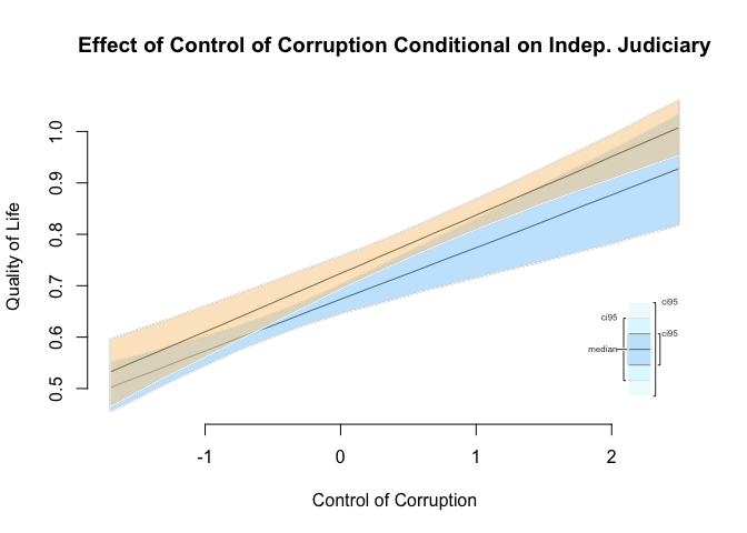
Comparing the two models we see that there is an effect of control of corruption on the quality of life. The better the institutions (more control of corruption), the higher the quality of life. We test the theory that the effect of control of corruption is conditional on having an independent judiciary, i.e. the magnitude of the effect is different in the two sub-groups. Our interaction term is insignificant. The effect of control of corruption seems to be independent of whether an independent judiciary exists or not. Our F-test also clearly rejects that our model with the interaction is doing better at explaining quality of life.
Normally, we would stop here. There is no point in illustrating a conditional effect that does not exist. However, below we illustrate the effect of control of corruption conditional on having an independent judiciary. The effects overlap and we cannot tell a difference.
Note: The interpretation relies on statistical significance. We do not find support for the conditional effect of X on Y.
z.out <- zelig(hdi ~ corruption_control * indep_judiciary,
               data = qog_data, model = "ls")
How to cite this model in Zelig:
  R Core Team. 2007.
  ls: Least Squares Regression for Continuous Dependent Variables
  in Christine Choirat, James Honaker, Kosuke Imai, Gary King, and Olivia Lau,
  "Zelig: Everyone's Statistical Software," http://zeligproject.org/
summary(qog_data$corruption_control)
    Min.  1st Qu.   Median     Mean  3rd Qu.     Max.     NA's
-1.70000 -0.81960 -0.30480 -0.05072  0.50650  2.44600        2
x.out1 <- setx(z.out, indep_judiciary = 0, corruption_control = seq(-1.7, 2.5, 0.1) )
x.out2 <- setx(z.out, indep_judiciary = 1, corruption_control = seq(-1.7, 2.5, 0.1) )

s.out <- sim(z.out, x.out1, x.out2)

# plot results
ci.plot(s.out,
        ci = 95,
        main = "Effect of Control of Corruption Conditional on Indep. Judiciary",
        xlab = "Control of Corruption",
        ylab = "Quality of Life")
Exercise 4
Clear your workspace and download the California Test Score Data used in Chapters 4-9 by Stock and Watson.
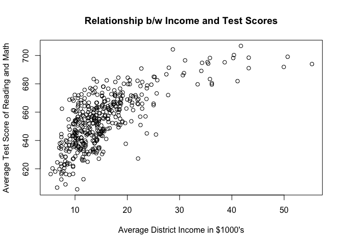
- Draw a scatterplot between district income and test scores.
- Run two regressions. One with and one without quadratic income.
- Test whether the quadratic model fits the data better.
Solution
Clear workspace
rm(list = ls())
Load the dataset and plot district income against test scores
ca_schools <- read.dta("caschool.dta")

# scatter plot
plot(testscr ~ avginc, data = ca_schools,
     main = "Relationship b/w Income and Test Scores",
     xlab = "Average District Income in $1000's",
     ylab = "Average Test Score of Reading and Math")
Estimate the two models -- one with quadratic income, and one without
model1 <- lm(testscr ~ avginc, data = ca_schools)
model2 <- lm(testscr ~ avginc + I(avginc^2), data = ca_schools)

screenreg(list(model1, model2))
===================================
             Model 1     Model 2
-----------------------------------
(Intercept)  625.38 ***  607.30 ***
              (1.53)      (3.05)
avginc         1.88 ***    3.85 ***
              (0.09)      (0.30)
I(avginc^2)               -0.04 ***
                          (0.01)
-----------------------------------
R^2            0.51        0.56
Adj. R^2       0.51        0.55
Num. obs.    420         420
RMSE          13.39       12.72
===================================
*** p < 0.001, ** p < 0.01, * p < 0.05
In both the models, average district income is statistically significant. Students from richer districts do better. Our quadratic term is also significant in the second model. Thus, the effect is stronger for poorer districts and smaller for richer districts. The F-test confirms that our non-linear model does better at explaining test scores.
anova(model1, model2)
Analysis of Variance Table

Model 1: testscr ~ avginc
Model 2: testscr ~ avginc + I(avginc^2)
  Res.Df   RSS Df Sum of Sq      F    Pr(>F)
1    418 74905
2    417 67510  1    7394.9 45.677 4.713e-11 ***
---
Signif. codes:  0 '***' 0.001 '**' 0.01 '*' 0.05 '.' 0.1 ' ' 1
We can go a step further and compare the effects of income increase in richer vs poorer districts.
Let's see what happens when we move from 10th percentile to 15th percentile of income:
z.out <- zelig(testscr ~ avginc + I(avginc^2), data = ca_schools, model = "ls")
How to cite this model in Zelig:
  R Core Team. 2007.
  ls: Least Squares Regression for Continuous Dependent Variables
  in Christine Choirat, James Honaker, Kosuke Imai, Gary King, and Olivia Lau,
  "Zelig: Everyone's Statistical Software," http://zeligproject.org/
x.low <- setx(z.out, avginc = quantile(ca_schools$avginc, 0.10))
x.high <- setx(z.out, avginc = quantile(ca_schools$avginc, 0.15))

s.out <- sim(z.out, x.low, x.high)
summary(s.out)
 sim x :
 -----
ev
      mean       sd      50%     2.5%    97.5%
1 638.2858 1.019334 638.2767 636.3581 640.2284
pv
         mean       sd      50%     2.5%    97.5%
[1,] 637.9882 12.81654 638.2065 611.6127 662.5857

 sim x1 :
 -----
ev
      mean        sd      50%     2.5%    97.5%
1 640.8613 0.9015329 640.8714 639.1829 642.5643
pv
         mean       sd      50%     2.5%    97.5%
[1,] 640.8461 12.83206 640.9189 615.7214 664.4534
fd
     mean        sd      50%     2.5%    97.5%
1 2.57554 0.1648453 2.580249 2.261046 2.892726
The simulation shows that the effect of moving from the 10th percentile in district wealth to the 15th percentile is 2.58 points. The difference is statistically significant, we can say that on a 95% confidence level test scores would increase between 2.26 and 2.89 points.
The difference in income between the 10th percentil and 15th percentile is roughly $840. Remember that the income is reported in x1000 US dollars, so we multiply the difference by 1000 to get the dollar amount:
quantile(ca_schools$avginc, c(0.10, 0.15))
     10%      15%
8.929933 9.770200
So the difference is 9.77 - 8.93 = 0.84 or $840.
We can also check for the effect that increasing income by the same amount ($840) would have in a wealthier district, for example let's say in the 75th percentile.
x.low <- setx(z.out, avginc = quantile(ca_schools$avginc, 0.75))
x.high <- setx(z.out, avginc = quantile(ca_schools$avginc, 0.75) + 0.84)

s.out <- sim(z.out, x.low, x.high)

summary(s.out)
 sim x :
 -----
ev
      mean        sd      50%     2.5%    97.5%
1 662.0423 0.8242851 662.0282 660.5017 663.6549
pv
         mean       sd      50%     2.5%    97.5%
[1,] 661.8853 12.50672 661.4153 637.9642 687.1944

 sim x1 :
 -----
ev
      mean        sd      50%     2.5%    97.5%
1 663.9952 0.8781278 663.9976 662.3599 665.7192
pv
       mean       sd      50%     2.5%    97.5%
[1,] 664.18 12.43611 663.8773 639.6473 688.6908
fd
      mean         sd      50%     2.5%    97.5%
1 1.952878 0.09072237 1.951245 1.776513 2.137769
When a district at the 75th percentile would become even richer by $840 average income, that would increase test scores by 1.95 points on average. On a 95% confidence level the increase would between 1.78 and 2.14 points. That effect is smaller than in poor districts.
Note: Here, the effect of X on Y was presented in the absolute change (point change of test scores) in this exercise as opposed to percentage increase as we did in previous examples. When the absolute increase of the dependent variable is easy to understand it is good to do that.