Introduction to Quantitative Methods

6. Assumptions and Violations of Assumptions

6.2 Solutions

Exercise 1

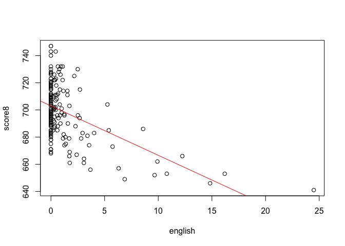
Fit a model to explain the relationship between percentage of english learners and average 8th grade scores.

Solution

Let's start by clearing the environment

rm(list = ls())

Next, we load the texreg, lmtest, sandwich and dplyr packages

library(lmtest)
library(sandwich)
library(texreg)
library(dplyr)

Load the dataset

MA_schools <- read.csv("MA_Schools.csv")

Now, we can run the linear model

model1 <- lm(score8 ~ english, data = MA_schools)
summary(model1)

Call:
lm(formula = score8 ~ english, data = MA_schools)

Residuals:
    Min      1Q  Median      3Q     Max 
-35.604 -12.763  -2.033  13.008  44.008 

Coefficients:
            Estimate Std. Error t value Pr(>|t|)    
(Intercept) 702.9918     1.4411 487.801  < 2e-16 ***
english      -3.6412     0.4352  -8.367 1.68e-14 ***
---
Signif. codes:  0 '***' 0.001 '**' 0.01 '*' 0.05 '.' 0.1 ' ' 1

Residual standard error: 17.89 on 178 degrees of freedom
  (40 observations deleted due to missingness)
Multiple R-squared:  0.2823,    Adjusted R-squared:  0.2782 
F-statistic: 70.01 on 1 and 178 DF,  p-value: 1.678e-14

According to our model, one unit increase in english learners in a school district has the effect of lowering the score by 3.64.

Exercise 2

Plot the model and the regression line

Solution

We create the scatter plot with the plot() function and add the regression line with abline()

plot(score8 ~ english, data = MA_schools)
abline(model1, col = "red")

Exercise 3

Check for correlation between the variables listed above to see if there are other variables that should be included in the model.

• HINT: There are some missing values in the dataset. Add the use = "complete.obs" or use = "pairwise.complete.obs" argument when calling the cor() function. Use online help for more details.

Solution

First let's take a look at the variables of interest and see if there are any missing values

summary(select(MA_schools, score8, stratio, english, lunch, income))

     score8         stratio         english            lunch      
 Min.   :641.0   Min.   :11.40   Min.   : 0.0000   Min.   : 0.40  
 1st Qu.:685.0   1st Qu.:15.80   1st Qu.: 0.0000   1st Qu.: 5.30  
 Median :698.0   Median :17.10   Median : 0.0000   Median :10.55  
 Mean   :698.4   Mean   :17.34   Mean   : 1.1177   Mean   :15.32  
 3rd Qu.:712.0   3rd Qu.:19.02   3rd Qu.: 0.8859   3rd Qu.:20.02  
 Max.   :747.0   Max.   :27.00   Max.   :24.4939   Max.   :76.20  
 NA's   :40                                                       
     income      
 Min.   : 9.686  
 1st Qu.:15.223  
 Median :17.128  
 Mean   :18.747  
 3rd Qu.:20.376  
 Max.   :46.855  

There are 40 missing values or NA in score8. Let's see what happens if we try to calculate the correlation between variables when there are some missing values in the dataset.

cor(select(MA_schools, score8, stratio, english, lunch, income))

        score8    stratio    english      lunch     income
score8       1         NA         NA         NA         NA
stratio     NA  1.0000000  0.1623002  0.1807368 -0.1566277
english     NA  0.1623002  1.0000000  0.6622803 -0.2379802
lunch       NA  0.1807368  0.6622803  1.0000000 -0.5626636
income      NA -0.1566277 -0.2379802 -0.5626636  1.0000000

The cor() function just gives us NA whenever one of the variables has missing values in it. To get around this problem, we can tell cor() to only use complete observations.

cor(select(MA_schools, score8, stratio, english, lunch, income), 
    use = "pairwise.complete.obs")

            score8    stratio    english      lunch     income
score8   1.0000000 -0.3164449 -0.5312991 -0.8337520  0.7765043
stratio -0.3164449  1.0000000  0.1623002  0.1807368 -0.1566277
english -0.5312991  0.1623002  1.0000000  0.6622803 -0.2379802
lunch   -0.8337520  0.1807368  0.6622803  1.0000000 -0.5626636
income   0.7765043 -0.1566277 -0.2379802 -0.5626636  1.0000000

Both lunch and income are highly correlated with score8. They also have the highest correlation with the independent variable english we used in the first model. Without these two variables, our model likely suffers from omitted variable bias.

Exercise 4

Add two variables from the list above that are highly correlated with both the independent and the dependent variable and run linear regression again.

Solution

Let's add the two variables lunch and income that we identified in the previous exercise and run linear regression again:

model2 <- lm(score8 ~ english + lunch + income, data = MA_schools)
summary(model2)

Call:
lm(formula = score8 ~ english + lunch + income, data = MA_schools)

Residuals:
    Min      1Q  Median      3Q     Max 
-20.748  -5.708  -1.051   5.173  31.945 

Coefficients:
             Estimate Std. Error t value Pr(>|t|)    
(Intercept) 678.59026    3.45214 196.571   <2e-16 ***
english      -0.25028    0.30738  -0.814    0.417    
lunch        -0.72428    0.06996 -10.353   <2e-16 ***
income        1.69515    0.14760  11.485   <2e-16 ***
---
Signif. codes:  0 '***' 0.001 '**' 0.01 '*' 0.05 '.' 0.1 ' ' 1

Residual standard error: 8.799 on 176 degrees of freedom
  (40 observations deleted due to missingness)
Multiple R-squared:  0.8283,    Adjusted R-squared:  0.8253 
F-statistic: 282.9 on 3 and 176 DF,  p-value: < 2.2e-16

Exercise 5

Compare the two models. Did the first model suffer from omitted variable bias?

Solution

screenreg(list(model1, model2))

===================================
             Model 1     Model 2   
-----------------------------------
(Intercept)  702.99 ***  678.59 ***
              (1.44)      (3.45)   
english       -3.64 ***   -0.25    
              (0.44)      (0.31)   
lunch                     -0.72 ***
                          (0.07)   
income                     1.70 ***
                          (0.15)   
-----------------------------------
R^2            0.28        0.83    
Adj. R^2       0.28        0.83    
Num. obs.    180         180       
RMSE          17.89        8.80    
===================================
*** p < 0.001, ** p < 0.01, * p < 0.05

The percentage of english learners is no longer significant once we control for average district income and students receiving lunch subsidy.

Exercise 6

Plot the residuals against the fitted values from the second model to visually check for heteroskedasticity.

Solution

We can plot the residuals against the fitted values exactly the same way we did that in the seminar

plot(fitted(model2), residuals(model2))

It's not clear from this plot whether our model suffers from heteroskedasticity.

Exercise 6

Run Breusch-Pagan Test to see whether the model suffers from heteroskedastic errors.

Solution

We use the bptest() function from the lmtest package to test for heteroskedasticity

bptest(model2)

    studentized Breusch-Pagan test

data:  model2
BP = 2.3913, df = 3, p-value = 0.4953

The p-value is quite high so we cannot reject the null hypothesis. Remember that the null hypothesis for the Breusch-Pagan test is that the variance of the error term is constant.

Exercise 7

Correct for heteroskedasticity (if needed) and present the results with corrected standard errors and p-values.

Solution

The model doesn't suffer from heteroskedastic errors so we don't need to do anything further. If the p-value from bptest() was less than 0.05 then we would have to correct for heteroskedastic errors using coeftest() and vcovHC() just like we did in the seminar.