Introduction to Quantitative Methods

5. Multiple linear regression models

5.2 Solutions

library(Zelig) 
library(texreg)

# clear workspace
rm(list = ls())

Exercise 1

1. Download the data from http://uclspp.github.io/PUBLG100/data/corruption.csv and read it in R.

Solution

# load csv data set
corruption_data <- read.csv("corruption.csv")

Exercise 3

Inspect the data. Spending some time here will help you for the next tasks. Knowing and understanding your data will help you when running and interpreting models and you are less prone to making mistakes.

Solution

There are many different ways to get an overview over the data. The important thing is that you know the levels of measurement and that you are roughly familiar with the range of the variables.

summary(corruption_data)

      country     country.code    country.abbr     ti.cpi     
 Albania  :  1   Min.   :  8.0   AGO    :  1   Min.   :1.200  
 Algeria  :  1   1st Qu.:209.0   ALB    :  1   1st Qu.:2.500  
 Angola   :  1   Median :420.0   ARE    :  1   Median :3.300  
 Argentina:  1   Mean   :431.5   ARG    :  1   Mean   :4.051  
 Armenia  :  1   3rd Qu.:658.0   ARM    :  1   3rd Qu.:4.900  
 Australia:  1   Max.   :894.0   AUS    :  1   Max.   :9.700  
 (Other)  :164                   (Other):164                  
      gdp             region  
 Min.   :  520   Africa  :51  
 1st Qu.: 1974   Americas:32  
 Median : 5280   Asia    :48  
 Mean   : 8950   Europe  :39  
 3rd Qu.:10862                
 Max.   :61190                

Exercise 4

Run a regression on gdp. Use ti.cpi (corruption perceptions index, larger values mean less corruption) and region as independent variables. Print the model results to a world file called model1.doc. Also print your output to the screen.

Region is a categorical variable and R recognizes it as a factor variable. The variable has four categories corresponding to the four regions. When you run the model, the regions are included as binary variables (also sometimes called dummies) that take the values 0 or 1. For example, regionAmericas is 1 when the observation (the country) is from the Americas. Only three regions are included in the model, while the fourth is what we call the baseline or reference category. It is included in the intercept. Interpreting the intercept would mean, looking at an African country when ti.cpi is zero. If the estimate for the region dummy Europe is significant then that means that there is a difference in the dependent variable between European countries and the baseline category Africa.

Solution

model1 <- lm(gdp ~ ti.cpi + region, data = corruption_data)

htmlreg(model1, file = "model1.doc")

The table was written to the file 'model1.doc'.

screenreg(model1)

============================
                Model 1     
----------------------------
(Intercept)     -6607.83 ***
                 (992.80)   
ti.cpi           3437.55 ***
                 (221.40)   
regionAmericas    104.63    
                (1243.02)   
regionAsia       1036.41    
                (1103.24)   
regionEurope     5758.61 ***
                (1287.72)   
----------------------------
R^2                 0.72    
Adj. R^2            0.71    
Num. obs.         170       
RMSE             5375.97    
============================
*** p < 0.001, ** p < 0.01, * p < 0.05

Exercise 5

Does the inclusion of region improve model fit compared to a model without regions but with the corruption perceptions index? Hint: You need to compare two models.

Solution

To do this, we estimate a model with ti.cpi but without the regions. We then run an F-test comparing the the two models. Taking a look at the p-value reveals we can reject the null hypothesis that the reduction in the unexplained error is due to chance. Our model including regions is an improvement over the more general model.

model2 <- lm(gdp ~ ti.cpi, data = corruption_data)

anova(model1, model2)

Analysis of Variance Table

Model 1: gdp ~ ti.cpi + region
Model 2: gdp ~ ti.cpi
  Res.Df        RSS Df  Sum of Sq      F    Pr(>F)    
1    165 4768671746                                   
2    168 5504948435 -3 -736276689 8.4919 2.802e-05 ***
---
Signif. codes:  0 '***' 0.001 '**' 0.01 '*' 0.05 '.' 0.1 ' ' 1

Exercise 6

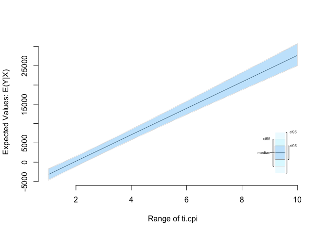
Predict gdp by varying ti_cpi from lowest to highest using the model that includes region. Plot your results.

Solution

We do this using zelig(). First, we estimate a linear model. Then we check the range of ti.cpi which varies roughly from 1 to 10. Then we set our covariates. And vary ti.cpi from 1 to 10. Next, we simulate using our model and the covariates and finally plot our predictions.

# estimate the linar model including regions
z.out <- zelig(gdp ~ ti.cpi + region, data = corruption_data, model = "ls")

How to cite this model in Zelig:
  R Core Team. 2007.
  ls: Least Squares Regression for Continuous Dependent Variables
  in Christine Choirat, James Honaker, Kosuke Imai, Gary King, and Olivia Lau,
  "Zelig: Everyone's Statistical Software," http://zeligproject.org/

# look at the ti.cpi variable to see the range
summary(corruption_data$ti.cpi)

   Min. 1st Qu.  Median    Mean 3rd Qu.    Max. 
  1.200   2.500   3.300   4.051   4.900   9.700 

# set the covariates
x.out <- setx(z.out, ti.cpi = 1:10)

# simulate
s.out <- sim(z.out, x.out)

ci.plot(s.out, ci = 95)

Exercise 7

Is there a difference between Europe and the Americas? Hint: is the difference between the predicted values for the two groups significantly different from zero?

Solution

We use zelig just like in exercise 6 but this time we set two specific scenarios. The first is Europe, the second is the Americas. Because ti.cpi is interval scaled and we did not specify a value for it, Zelig automatically sets it to the mean. Once we simulated, we look at the first differences and can confirm that the difference in political stability between the two regions is indeed statistically different from zero.

# estimate the linear model including regions
z.out <- zelig(gdp ~ ti.cpi + region, data = corruption_data, model = "ls")

How to cite this model in Zelig:
  R Core Team. 2007.
  ls: Least Squares Regression for Continuous Dependent Variables
  in Christine Choirat, James Honaker, Kosuke Imai, Gary King, and Olivia Lau,
  "Zelig: Everyone's Statistical Software," http://zeligproject.org/

# look at the labels of the factor variable regions
table(corruption_data$region)

  Africa Americas     Asia   Europe 
      51       32       48       39 

# set the covariates
x.out.europe <- setx( z.out, region = "Europe")
x.out.americas <- setx( z.out, region = "Americas")

# simulate
s.out <- sim( z.out, x = x.out.europe, x1 = x.out.americas)

# look at the first difference
summary(s.out)

 sim x :
 -----
ev
      mean       sd      50%    2.5%   97.5%
1 13060.62 961.9887 13046.78 11234.2 14987.8
pv
         mean       sd      50%     2.5%    97.5%
[1,] 13210.96 5607.429 13218.35 2564.812 24437.27

 sim x1 :
 -----
ev
      mean       sd      50%     2.5%    97.5%
1 7433.888 932.3523 7438.061 5614.709 9292.553
pv
         mean       sd      50%      2.5%   97.5%
[1,] 7427.308 5427.784 7588.531 -3039.745 17687.2
fd
       mean       sd       50%      2.5%     97.5%
1 -5626.731 1322.172 -5611.846 -8131.024 -2977.588