Introduction to Quantitative Methods

4. Bivariate linear regression models

4.2 Solutions

library(texreg)
library(Zelig)
library(dplyr)

# Change your working directory
setwd("N:/PUBLG100")

# Check your working directory
getwd()

# clear the environment
rm(list = ls())

Exercise 1

Download the CABenefits.csv from the link below and merge it with the CAStudents.csv dataset.

Solution

Let's read the two datasets and see if there are any variables common between the two datasets:

CA_benefits <- read.csv("CABenefits.csv")
CA_students <- read.csv("CAStudents.csv")

head(CA_benefits)

  district calworks   lunch
1    75119   0.5102  2.0408
2    61499  15.4167 47.9167
3    61549  55.0323 76.3226
4    61457  36.4754 77.0492
5    61523  33.1086 78.4270
6    62042  12.3188 86.9565

head(CA_students)

   county                          school  read  math
1 Alameda              Sunol Glen Unified 691.6 690.0
2   Butte            Manzanita Elementary 660.5 661.9
3   Butte     Thermalito Union Elementary 636.3 650.9
4   Butte Golden Feather Union Elementary 651.9 643.5
5   Butte        Palermo Union Elementary 641.8 639.9
6  Fresno         Burrel Union Elementary 605.7 605.4

The CA_benefits dataset identifies a school by it's district ID while CA_students uses the school name and county. That means that we cannot directly merge these two datasets without some help. Fortunately, the CA_admin dataset from the seminar can be used to match district ID with school and county. So, let's merge the CA_admin dataset to CA_students first and then bring in the CA_benefits dataset.

CA_admin <- read.csv("CASchoolAdmin.csv")

CA_schools <- merge(CA_admin, CA_students, by = c("county", "school"))
CA_schools <- merge(CA_schools, CA_benefits, by = "district")

head(CA_schools)

  district county                          school grades students teachers
1    61382  Butte         Bangor Union Elementary  KK-08      146     8.00
2    61457  Butte Golden Feather Union Elementary  KK-08      243    14.00
3    61499  Butte            Manzanita Elementary  KK-08      240    11.15
4    61507  Butte        Oroville City Elementary  KK-08     3401   175.55
5    61523  Butte        Palermo Union Elementary  KK-08     1335    71.50
6    61549  Butte     Thermalito Union Elementary  KK-08     1550    82.90
  computer expenditure    income   english  read  math calworks   lunch
1       34    6231.602  7.105000  0.000000 646.1 629.8  25.3425 54.1096
2       85    7101.831  8.978000  0.000000 651.9 643.5  36.4754 77.0492
3      101    5099.381  9.824000  4.583333 660.5 661.9  15.4167 47.9167
4      560    5489.589 11.266125 16.171715 641.5 638.1  52.2199 74.2723
5      171    5235.988  9.080333 13.857677 641.8 639.9  33.1086 78.4270
6      169    5501.955  8.978000 30.000002 636.3 650.9  55.0323 76.3226

Exercise 2

Estimate a model explaining the relationship between test scores and the percentage qualifying for CalWorks income assistance?

Solution

Let's create the score variable first just like we did in the seminar

CA_schools <- mutate(CA_schools, score = (math + read) / 2)

Next, use lm() to fit a linear model.

calworks_model <- lm(score ~ calworks, data = CA_schools)

summary(calworks_model)

Call:
lm(formula = score ~ calworks, data = CA_schools)

Residuals:
    Min      1Q  Median      3Q     Max 
-49.573  -9.583   0.239   9.216  39.902 

Coefficients:
             Estimate Std. Error t value Pr(>|t|)    
(Intercept) 667.96786    1.10949  602.05   <2e-16 ***
calworks     -1.04267    0.06339  -16.45   <2e-16 ***
---
Signif. codes:  0 '***' 0.001 '**' 0.01 '*' 0.05 '.' 0.1 ' ' 1

Residual standard error: 14.86 on 418 degrees of freedom
Multiple R-squared:  0.3929,    Adjusted R-squared:  0.3915 
F-statistic: 270.6 on 1 and 418 DF,  p-value: < 2.2e-16

screenreg(calworks_model)

=======================
             Model 1   
-----------------------
(Intercept)  667.97 ***
              (1.11)   
calworks      -1.04 ***
              (0.06)   
-----------------------
R^2            0.39    
Adj. R^2       0.39    
Num. obs.    420       
RMSE          14.86    
=======================
*** p < 0.001, ** p < 0.01, * p < 0.05

Exercise 3

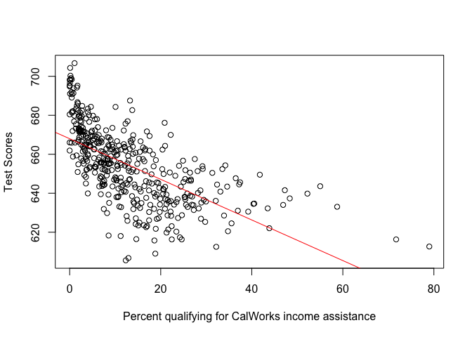
Plot the regression line of the model.

Solution

Plot the observations and a regression line.

plot(score ~ calworks, 
     data = CA_schools,
     xlab = "Percent qualifying for CalWorks income assistance",
     ylab = "Test Scores")

abline(calworks_model, col = "red")

Exercise 4

How does this model compare to the models we estimated in the seminar with STR and income as independent variables? Present your findings by comparing the output of all three models in side-by-side tables using the texreg package.

Solution

First, let's create a student-teacher ratio variable so we can estimate the first model from the seminar.

CA_schools <- mutate(CA_schools, STR = students/teachers)

Now, estimate the two models

STR_model <- lm(score ~ STR, data = CA_schools)

income_model <- lm(score ~ income, data = CA_schools)

screenreg(list(STR_model, income_model, calworks_model))

===============================================
             Model 1     Model 2     Model 3   
-----------------------------------------------
(Intercept)  698.93 ***  625.38 ***  667.97 ***
              (9.47)      (1.53)      (1.11)   
STR           -2.28 ***                        
              (0.48)                           
income                     1.88 ***            
                          (0.09)               
calworks                              -1.04 ***
                                      (0.06)   
-----------------------------------------------
R^2            0.05        0.51        0.39    
Adj. R^2       0.05        0.51        0.39    
Num. obs.    420         420         420       
RMSE          18.58       13.39       14.86    
===============================================
*** p < 0.001, ** p < 0.01, * p < 0.05

Exercise 5

Save your model comparison table to a Microsoft Word document (or another format if you don't use Word).

Solution

Save the output to a document using htmlreg()

htmlreg(list(STR_model, income_model, calworks_model), 
        file = "solutions4_model_comparison.doc")

The table was written to the file 'solutions4_model_comparison.doc'.

Exercise 6

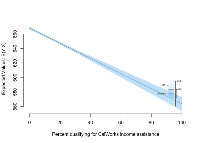
Generate predicted values from the fitted model with calworks and plot the confidence interval using Zelig.

Solution

This follows the example exactly as we covered in the seminar. We first estimate the model with zelig(), then generate predicted values with setx() and sim().

Let's check the range of values for the calworks variable:

range(CA_schools$calworks)

[1]  0.0000 78.9942

Since calworks is a percentage, we'll just use a range from 0 to 100 and increment it by 0.5. There's nothing special about 0.5 here, but just remember that the smaller the number, the more scenarios Zelig will attempt to simulate.

z.out <- zelig(score ~ calworks, data = CA_schools, model = "ls")

How to cite this model in Zelig:
  R Core Team. 2007.
  ls: Least Squares Regression for Continuous Dependent Variables
  in Christine Choirat, James Honaker, Kosuke Imai, Gary King, and Olivia Lau,
  "Zelig: Everyone's Statistical Software," http://zeligproject.org/

x.out <- setx(z.out, calworks = seq(0, 100, 0.5))
s.out <- sim(z.out, x = x.out)

ci.plot(s.out, ci = 95, xlab = "Percent qualifying for CalWorks income assistance")

Exercise 8

Save all the plots as graphics files.

Solution

Use png() to send the plot to a file. When we're done plotting, we must close the file with dev.off()

png(filename = "solutions4_calworks_model.png")

plot(score ~ calworks,
     data = CA_schools,
     xlab = "Percent qualifying for CalWorks income assistance",
     ylab = "Test Scores")
abline(calworks_model, col = "red")

dev.off()

Now let's do the same for the confidence interval plot.

png(filename = "solutions4_calworks_model_zelig.png")

ci.plot(s.out, 
        ci = 95,
        xlab = "Percent qualifying for CalWorks income assistance",
        ylab = "Expected Value of Test Score")

dev.off()