Introduction to Quantitative Methods

1. Introduction to Quantitative Analysis

1.2 Solutions

rm( list = ls() )

Exercise 3) Check your working directory

getwd()

[1] "/Users/altaf/Projects/PUBLG100/week1"

Exercise 4) Change your working directory to your folder N:/PUBLG100

setwd("N:/PUBLG100")

Exercise 5) Create a vector with all even elements b/w 1 & 11 in ascending order

# assign the 5 elements to a
a <- c( 2, 4, 6, 8, 10)
# check what a contains
a

[1]  2  4  6  8 10

Exercise 6) Delete the last element from your vector

Solution 1: We use length().

1. length(a) returns the number of elements in a which is 5

2. we then assign a again indicated by the arrow

3. because a already existed we overwrite it

4. the square brackets after a tell you, we are subsetting a
5. so we overwrite a with a subset of a
6. the minus in the square bracket can be read as: except
7. so we overwrite a with the vector a except the element at position length(a) which is the last element

a <- a[- length(a)]
a

[1] 2 4 6 8

Solution 2 using head()

1. head() returns the first 6 elements, if you do not specify a number
2. If you specify a positive number x (after the comma), it returns the first x elements
3. If you specify a negative number x, it returns all elements except for the last x elements
4. You can use tail() to check last elements

We also create the vector a anew because we already deleted the last element in solution 1.

# create a again
a <- c( 2, 4, 6, 8, 10,4)
# delete last element
a <- head(a, -1)
# see what a contains now
a

[1]  2  4  6  8 10

Exercise 7) Create a square matrix with 3 rows and 3 columns.

1. row 1: smallest positive integers divisible by 3, in ascending order.
2. row 2: smallest prime numbers, in ascending order
3. row 3: greatest multiples of 6, smaller than 60, in descending order In R, there is usually more than one way to do something.

Solution 1: matrix()

matrix takes as necessary arguments, the data, the number of rows, and columns. You should always check the syntax of a command by typing: help(command.name) and see what is required.

# assign the values to the matrix
m <- matrix( c( 3, 6, 9, 2, 3, 5, 54, 48, 42), 3, 3, byrow = T)
# print the contents of m to the screen (check what m contains)
m

     [,1] [,2] [,3]
[1,]    3    6    9
[2,]    2    3    5
[3,]   54   48   42

Solution 2: rbind()

rbind() combines vectors (works also for matrices and data frames) row-wise. cbind() combines column-wise. In the example below c(3, 6, 9) is the first vector. c(2, 3, 5) is the second vector. c(54, 48, 42) is the third vector. These three vectors are combined row-wise with rbind().

# assing the values to the matrix
m <- rbind( c(3, 6, 9), c(2, 3, 5), c(54, 48, 42))
# check what m contains
m

     [,1] [,2] [,3]
[1,]    3    6    9
[2,]    2    3    5
[3,]   54   48   42

Exercise 8) Change the elements on the main diagonal to 1's

Again, there is more than one solution.

Solution 1: Manually assigning each element on the diagonal

# assign a 1 to row 1 and column 1 of m
m[1, 1] <- 1
# assign a 1 to row 2 and column 2 of m
m[2, 2] <- 1
# assign a 1 to row 3 and column 3 of m
m[3, 3] <- 1
# check what m contains
m

     [,1] [,2] [,3]
[1,]    1    6    9
[2,]    2    1    5
[3,]   54   48    1

Solution 2: The quick way using diag(). diag() returns the elements on the diagonal of a matrix. We will also assign the matrix again because we have already changed the diagonal of m in solution 1

# assigning the values from Exercise 7 to m again
m <- rbind( c(3, 6, 9), c(2, 3, 5), c(54, 48, 42))
# assigning a 1 to each element on the diagonal of m
diag(m) <- 1
# checking what m contains
m

     [,1] [,2] [,3]
[1,]    1    6    9
[2,]    2    1    5
[3,]   54   48    1

Exercise 9) Load "polity.csv" and call your data frame "df"

We use read.csv which reads in standard comma separated files.

# assign the csv file to df
df <- read.csv("http://uclspp.github.io/PUBLG100/data/polity.csv")

Exercise 10) Pick the year 1991 and drop all observations from the data set that are not from 1991.

# assign(overwrite) df to df but only those rows where 
# the variable year is equal to 1991
df <- df[ df$year == 1991, ]
# look at the first 6 rows of data set df
head(df)

     id scode                          country year polity2 democ nato
192 192   AFG Afghanistan                      1991      -8     0    0
293 293   ALB Albania                          1991       1     3    0
346 346   ALG Algeria                          1991      -2     1    0
386 386   ANG Angola                           1991      -3   -88    0
576 576   ARG Argentina                        1991       7     7    0
600 600   ARM Armenia                          1991       7     7    0

Exercise 11) Summarise the variable democ (stands for democracy) and produce a frequency table.

# summary() returns summary statistics
# the $ indicates that you want to access something in data set df
# in this case the variable democ
summary( df$democ)

   Min. 1st Qu.  Median    Mean 3rd Qu.    Max. 
-88.000   0.000   3.000  -3.155   8.000  10.000 

# table() produces a frequency table
table(df$democ)

-88 -77 -66   0   1   2   3   4   5   6   7   8   9  10 
 10   3   1  52   8   4   3   3   6  12   8  14   8  29 

Exercise 12) Delete all observations from the data where democ is smaller than zero.

We do this by overwriting df again with the rows of df that we want to keep. Since we are asked to delete observations where democ is smaller than zero, we want to keep observations where democ is greater or equal to zero. We use a logical operator to do this: >= which means greater or equal. Common logical operators:

1. == equal to
2. != not equal to
3. > greater
4. >= greater or equal
5. < smaller
6. <= smaller or equal
7. is.na() is missing

# assign (overwrite in this case) df with df but only those rows (observations)
# of df where democracy is greater or equal to zero
df <- df[ df$democ >= 0, ]

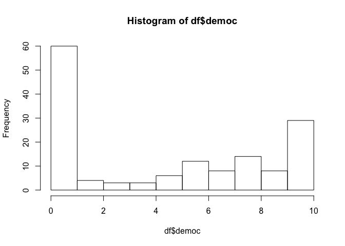
Exercise 13) Print a histogram of the democ (type help("hist").

hist( df$democ)