1 Introduction

Measuring several single grain U-Th-(Sm)-He aliquots per sample is not only possible, thanks to the development of laser heating (House et al., 2000), but also desirable, because U-Th-(Sm)-He data are generally overdispersed with respect to the formal analytical uncertainty and this overdispersion can only be quantified by analysing a representative number of mineral grains. The question then arises how to average these measurements. Traditionally, this is done by simply averaging the single grain age estimates, an ad hoc solution that lacks a proper theoretical justification and does not make full use of the data. Potentially valuable information is lost when the chemical composition of samples is ignored, and compositional controls on thermochronological models may go unnoticed. The most natural way to study U-Th-(Sm)-He data is as a geochemical composition on a ternary diagram or in logratio space (Vermeesch, 2008).

HelioPlot is a data visualisation tool that plots U-Th-(Sm)-He data on ternary diagrams and logratio plots. The program also calculates the so-called ‘central age’, which is the age corresponding to the geometric mean U-Th-(Sm)-He composition. To this end, it applies a weighted mean algorithm taking into account both the analytical uncertainty and any possible overdispersion simultaneously, in contrast with Vermeesch (2008)’s web calculator, which propagated them separately. U-Th-(Sm)-He data are often overdispersed with respect to the analytical uncertainty, for reasons that have been discussed elsewhere (Fitzgerald et al., 2006; Shuster et al., 2006). The amount of overdispersion can be quantified using the Mean Square of the Weighted Deviates (MSWD,  McIntyre et al., 1966). Given a dataset of n age measurements, or the logarithms thereof (t_i, for 1≤i≤n), the MSWD is a measure of the ratio of the observed scatter of the data points (t_i) around the mean value (t) to the expected scatter from the assigned errors (σ_i):

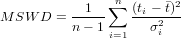(1)

If the assigned errors are the only cause of scatter, the MSWD will tend to be near unity. MSWD values much less than unity indicate either overestimated analytical errors or unrecognized error-correlations. MSWD values much greater than unity generally indicate either underestimated analytical errors, or the presence of non-analytical scatter. HelioPlot implements methods to deal with the latter situation.

Although there is no formally agreed convention for calculating the average of multiple (U-Th)/He ages, this is either done by computing the unweighted arithmetic mean, ignoring the analytical precision, or by calculating the error-weighted mean, ignoring overdispersion. Section 2 introduces a one-dimensional weighted mean algorithm that deals with analytical precision and overdispersion simultaneously, using the method of maximum likelihood. Section 3 generalises this method to compositional data space, so as to calculate the best estimate for the central age, taking into account both the internal and external reproducibilities of the data, as well as their full covariance structure. ‘Conventional’ propagation of uncertainty for the central age, as implemented by Vermeesch (2008), involves linearisation by a first-order Maclaurin series expansion, which may be inaccurate. Section 4 proposes a deterministic algorithm to avoid this problem, yielding exact confidence intervals for the central age. Finally, Section 5 provides further details about HelioPlot and illustrates its usefulness with a number of real world examples.

2 Overdispersed ages

Assume that the ages (or the logarithm of the ages) come from a normal distribution of the form

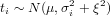(2)

where μ denotes the mean and ξ² is the amount of overdispersion, i.e. the excess scatter that cannot be explained by the analytical uncertainty alone. Unbiased estimates and ² for these two parameters can be obtained by maximising the likelihood l:

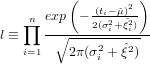(3)

or, more conveniently, the log-likelihood L ≡ log(l):

(4)

Calculating the derivatives of L with respect to and ² and setting them to zero to find the maximum likelihood:

	= ∑ i=1n = 0	(5)
	= ∑ i=1n = 0	(6)

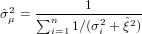
which can be solved iteratively for and ². The variance _μ² of the weighted mean is given by the inverse of the Fisher Information, i.e. the negative expected value of the second derivative of the log-likelihood function with respect to :

(7)

3 Overdispersed compositions

U, Th and He form a ternary system, can be plotted on a ternary diagram, and are subject to the peculiar mathematics of the ternary dataspace. The ‘central age’ is calculated from the geometric mean composition of a U-Th-(Sm)-He dataset and is a more accurate estimator of the true age than the arithmetic mean (Vermeesch, 2008). This concept can be easily generalised to four dimensions and this section will, therefore, discuss the case of (U-Th-Sm)/He dating. Given n single grain measurements [Uⁱ, Thⁱ, Smⁱ, Heⁱ] (1≤i≤n), the calculation of a central age involves a bijection from the four-dimensional ‘simplex’ to a three-dimensional Euclidean logratio-space (Aitchison, 1986; Vermeesch, 2008):

(8)

The central age is obtained by calculating the average logratio composition (v, w, x) and converting it to a geometric mean composition using the inverse logratio transformation:

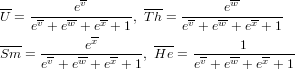(9)

This result is then plugged into the U-Th-(Sm)-He age equation.

The problem of averaging the compositions is very similar to the problem of averaging the ages discussed in the previous section. Given n logratio measurements Xⁱ and their (co)variances Eⁱ (1 ≤ i ≤ n):

(10)

our aim is to develop an algorithm to calculate the weighted mean M and its covariance matrix Σ:

(11)

In principle, the logratio covariances (Eⁱ) could be directly determined from the raw mass spectrometer measurements. In practice, however, they are calculated from the individual concentrations by linear approximation, using Equation 21 of Vermeesch (2008), which assumes that the errors on the individual concentrations are Normal and independently distributed. Rather than propagating the internal and external uncertainties separately, as done by Vermeesch (2008), this section introduces a weighted mean algorithm that considers both factors simultaneously, using a multivariate generalisation of the one-dimensional maximum likelihood algorithm developed in Section 2. First, redefine the MSWD in matrix form:

(12)

where df = d × (n - 1) is the number of degrees of freedom of the problem, with d = 2 for (U-Th)/He and d = 3 for (U-Th-Sm)/He dating. Note that, because the variability of Sm does not contribute as much to the age dispersion as that of U and Th, it is better to use only the latter two elements for the MSWD calculation. If MSWD ≫ 1, the data are overdispersed and, in analogy with Equation 2, we will assume that the observations come from a multivariate normal distribution of the form

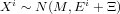(13)

where M denotes the mean and Ξ is the overdispersion. The log-likelihood is given by:

(14)

and can be found by solving the following system of non-linear equations:

	= ∑ i=1n[(Ei + )-1(Xi -)] = 0	(15)
	= ∑ i=1n[(Ei + )-1(Xi -)(Xi -)′(Ei + )-1 - (Ei + )-1] = 0	(16)

The covariance matrix of the weighted mean is obtained by inverting the Fisher Information matrix, i.e. the matrix of the negative expected values of the second derivatives of the log-likelihood function:

(17)

4 Confidence intervals

Using the covariance matrix of the logratio average (), and performing a linear error propagation, it is straightforward to calculate the covariance matrix of the geometric mean composition (), evaluated at :

(18)

where A is the matrix of first derivatives of Equation 9:

(19)

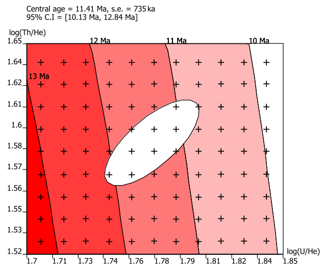
Equation 18 contains an expression for the covariances of the geometric mean composition, which were omitted by Vermeesch (2008) but are required for a full propagation of age uncertainty. However, even the complete error propagation may be inaccurate because it is based on a first order Maclaurin series expansion of Equation 9, which is highly non-linear. This problem can be circumvented using numerical techniques, such as the following deterministic algorithm. First, build a regular grid across the two (for U-Th-He) or three (for U-Th-Sm-He) dimensions of logratio space (Figure 1.a). Second, for each of these grid points, calculate (a) its likelihood under a normal distribution with mean and covariance matrix , and (b) the corresponding age. Third, calculate the Bayesian cumulative posterior distribution by ranking the numerical data in order of increasing age and computing the running sum of the likelihoods. Fourth, obtain an asymmetrical 95% confidence interval from the 2.5 and 97.5 percentiles of the posterior distribution (Figure 1.b).

a. b.

Figure 1: a. the deterministic Bayesian algorithm collects a large number of ages across a regular grid in logratio space (crosses), and records the corresponding logistic normal likelihood of the data (ellipse); b. 95% confidence intervals are then simply calculated by looking up the 2.5 and 97.5 percentiles of the resulting ‘posterior distribution’.

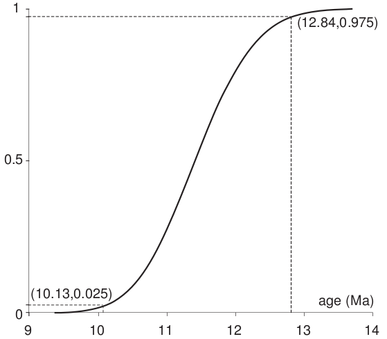
5 Applications

HelioPlot is a computer program for visualising U-Th-(Sm)-He data on ternary diagrams and logratio plots that implements all the above calculations, including the computation of central ages and 95% confidence intervals. Equations 6 and 16 are solved using Newton’s method. HelioPlot was written in Java and is, therefore, perfectly platform independent. The program and its source code can be downloaded free of charge from http://pvermees.andropov.org/helioplot. Data can be copied and pasted to-and-from Microsoft Excel, or entered directly using the built-in editing tools. Data files are saved in a comma-separated-variable (.csv) format. Samarium is an optional input parameter and the complete functionality of the program is still available when Sm is missing. If Sm is absent, it will be assumed to be zero, and the data naturally reduce to their two dimensions in compositional datapace. 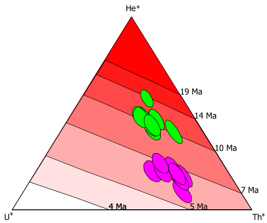If Sm is present, the geometric mean Sm composition is used as a common reference for the ternary diagrams and logratio plots. Colour is used to visualise the Sm content of aliquots, or any other numerical quantity, such as sample number (Figure 2.a), grain size (Figure 2.b), elevation, or, for the case of double-dated grains, a U-Pb or fission track age (Campbell et al., 2005). HelioPlot is capable of saving the graphical output as either bitmap or vector images, in a .png or .pdf format, respectively.

Example input files are provided on the website for testing purposes. Figure 2.b shows the output for one of these files, based on a published (U-Th)/He dataset (Vermeesch et al., 2007), which was α-ejection corrected according to the guidelines of Ketcham (2009). The output includes the arithmetic and geometric mean ages and their standard errors, calculated using the methods of Section 2, in addition to the central age, its standard error and 95% confidence interval, calculated according to the algorithm of Section 3. Three separate MSWDs are given, reflecting the overdispersion of the ages and the U-Th-He compositions.

a. b.

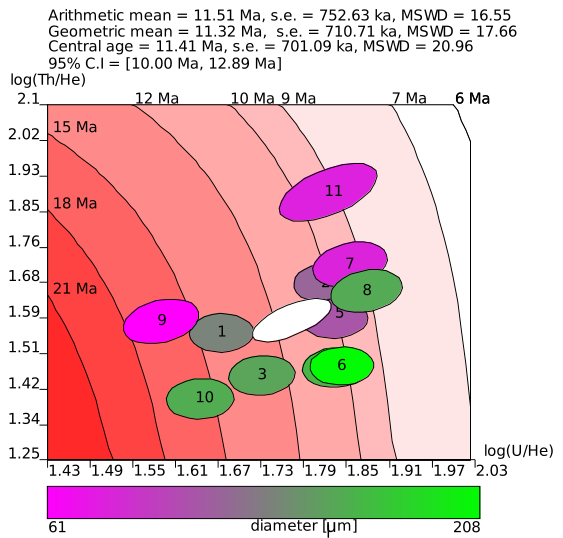
Figure 2: Two diagrams produced by HelioPlot. (a) Ternary diagram with two synthetic U-Th-He samples (U* = , Th* = , He* = ). (b) Logratio plot of U-Th-He data from Naxos (Vermeesch et al., 2007), colour-coded according to grain size. The geometric mean composition is shown as a white ellipse.

6 Conclusions

The aim of this paper was to bring the statistical treatment of U-Th-(Sm)-He data on an equal footing with more established geochronometers such as U-Pb, ⁴⁰Ar/³⁹Ar, or fission tracks. Weighted least squares algorithms similar to the maximum likelihood methods of Sections 2 and 3 have been used in U-Pb (Ludwig, 1998) and fission track dating (Galbraith and Green, 1990). Visual aids such as the U-Pb concordia diagram, the Rb-Sr isochron, or the fission track radial plot can be very useful for the exploratory analysis of geochronological data. The ternary diagram and logratio plot play the same role for helium thermochronology, as they bring out the full information content of U-Th-(Sm)-He data, and can help to reveal patterns between aliquots and samples that may not be seen otherwise.

Acknowledgments

John Rudge formulated equation 13, from which the rest of the calculations followed naturally. He and an anonymous reviewer are gratefully acknowledged for this and other constructive comments.

References

Aitchison, J., 1986. The statistical analysis of compositional data. London, Chapman and Hall.
Campbell, I. H., Reiners, P. W., Allen, C. M., Nicolescu, S., Upadhyay, R., Sep. 2005. He-Pb double dating of detrital zircons from the Ganges and Indus Rivers: Implication for quantifying sediment recycling and provenance studies. Earth and Planetary Science Letters 237, 402–432.
Fitzgerald, P. G., Baldwin, S. L., Webb, L. E., O’Sullivan, P. B., 2006. Interpretation of (U-Th)/He single grain ages from slowly cooled crustal terranes: A case study from the Transantarctic Mountains of southern Victoria Land. Chemical Geology 225, 91–120.
Galbraith, R. F., Green, P. F., 1990. Estimating the component ages in a finite mixture. Nuclear Tracks and Radiation Measurements 17, 197–206.
House, M. A., Farley, K. A., Stockli, D., Dec. 2000. Helium chronometry of apatite and titanite using Nd-YAG laser heating. Earth and Planetary Science Letters 183, 365–368.
Ketcham, R., 2009. Refinements for alpha stopping distances and FT corrections. OnTrack, the electronic newsletter of the international thermochronology community 16.
Ludwig, K. R., Feb. 1998. On the treatment of concordant uranium-lead ages. Geochimica et Cosmochimica Acta 62, 665–676.
McIntyre, G. A., Brooks, C., Compston, W., Turek, A., 1966. The Statistical Assessment of Rb-Sr Isochrons. Journal of Geophysical Research 71, 5459–5468.
Shuster, D. L., Flowers, R. M., Farley, K. A., Sep. 2006. The influence of natural radiation damage on helium diffusion kinetics in apatite. Earth and Planetary Science Letters 249, 148–161.
Vermeesch, P., 2008. Three new ways to calculate average (U-Th)/He ages. Chemical Geology 249, 339–347.
Vermeesch, P., Seward, D., Latkoczy, C., Wipf, M., Günther, D., Baur, H., 2007. α-Emitting mineral inclusions in apatite, their effect on (U-Th)/He ages, and how to reduce it. Geochimica et Cosmochimica Acta 71, 1737–1746.