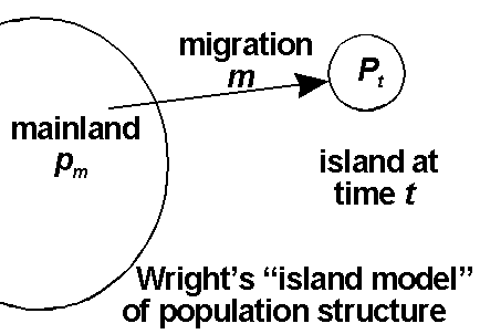
By population structure, population geneticists mean that, instead of a single, simple population, populations are subdivided in some way. The overall "population of populations" is often called a metapopulation, while the individual component populations are often called, well ... subpopulations, but also local populations, or demes. In fact, in many real populations, there may not be any obvious individual populations or substructure at all, and the populations are continuous. However, even in effectively continuous populations, different areas can have different gene frequencies, because the whole metapopulation is not panmictic. For instance, among humans, Scotland, the North of England, and London have some quite major language differences, suggesting substructure, but you would be hard put to find an exact boundary where there is a changeover. Such populations are structured, but continuously, in space.

A very good definition of population structure is when populations have deviations from Hardy-Weinberg proportions, or deviations from panmixia. If there is inbreeding, or selection, or if migration is important, then populations can be said to be structured in some way.

If populations are subdivided, they can evolve apart, somewhat independently. Population structure allows populations to diversify. This is the reason why population structure is a very important part of evolutionary genetics.

In this lecture we will deal with some simple models of how population structure and migration interferes with natural selection and drift to allow diversification.

Here, several topics are important:

1) Selection in a patchy environment (this can lead to a kind of migration/selection balance which favours polymorphism). To avoid interrupting the flow, we cover this in a separate page.  More is covered under the lecture Evolution in space and time).
2) The evolutionary effect of migration (gene flow) on its own.
3) How to measure population substructure using F_ST.
4) The possibility of drift/migration balance.

Gene flow (migration)

• homogenizes gene frequencies
• can reduce local adaptation, by preventing divergence (see separate lecture Evolution in Space and Time)

• Blacks in SE USA. Have different blood groups compared with the West Africans from which they originated.
• Convergence towards allele frequencies of Europeans.
• Suggests m ~ 0.01 - 0.04 per generation.

Subdivision into populations with distinct gene frequencies creates a heterozygote deficit due to subdivision into subpopulations (this can be considered a sort of inbreeding):

Example:
                              AA          Aa         aa

HW calcs:         pi           pi2        2piqi        qi2

Deme 1           0.75       0.5625      0.375       0.0625

Deme 2           0.25       0.0625      0.375       0.5625

Totals           1          0.625       0.75        0.625

Overall freqs.   0.5(=pav)   0.3125      0.375       0.3125

pav=fr(AA) + fr(Aa)/2=0.3125 + 0.375/2=0.5;
qav=(1-pav)=0.5

To find the heterozygote deficit, F:

2pavqav(1-F)=0.5(1-F)=0.375

Thus:

F=1-(0.375/0.5)=0.25

F_st can also be shown to be equal to the standardized variance of gene fequency (also called the Wahlund variance) in the n subpopulations, divided by (standardized by) the maximum possible variance, p_avq_av. The maximum possible variance is the variance when different populations are fixed for A or a (p_av is the average gene frequency over all subpopulations). In this case:

F_st=/(p_avq_av)={[(0.75-0.5)² + (0.25-0.5)²]/2} / 0.5x0.5=0.25

i.e. the same as we had by looking at the heterozygote deficit. In general it is true that this standardized variance of gene frequencies measures the heterozygote deficit due to subdivision over a number of populations and vice-versa.

Understanding F_st as a fraction of total variance is a useful one. F_st is the proportion of genetic variation found between as opposed to within each populations.  Thus (1-F_st) is the proportion of the total metapopulation genetic variation found within as opposed to between populations.  If there is a lot of local fixation or inbreeding, F_st will be near 1; if very little, F_st will be low (0.05, for instance, might be a typical value).

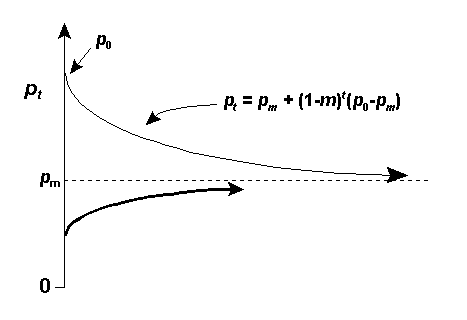
Migration (m) from the mainland can balance drift occurring on islands with small population sizes (N);

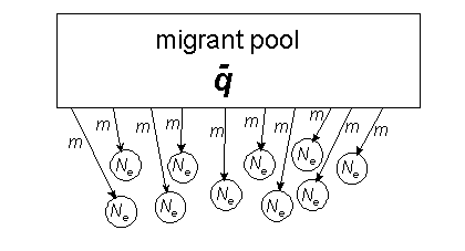
F_st ~ 1/(1+4Nm).  For the proof, CLICK HERE.

• If m << 1/N, then F~1
• If m >> 1/N, then F~0

PROBLEMS:

Island population structure: very unrealistic!
However, similar equations apply to more realistic structures, e.g. stepping stone models, continuous populations with limited migration.
So the island model is much USED (and also ABUSED!).

EXAMPLES

Population subdivision estimated from allele frequencies in some wild populations:
 

Organism                     No. pops.       No. loci            Fst     Nem
                                                                                                
High levels of gene flow x population size

Tobacco budworm moth
(Southeast USA)                 60              13              0.002   135

Intermediate levels of gene flow x population size

Human
(3 major "races")                3              35              0.069   3.4
(Yanomami villages)             37              15              0.077   3.0
(Italian villages)              34               3              0.035   6.9

Low levels of gene flow x population size

House mouse                      4              40              0.113   2.0
Kangaroo rat                     9              18              0.674   0.12

WRIGHT'S "ISOLATION BY DISTANCE MODEL" OF POPULATION STRUCTURE
(He made a lot of models, didn't he!)

Measuring dispersal

If the dispersal of an individual between place of birth and breeding site is essentially random, it resembles a "drunkards walk". You have probably encountered this sort of movement in physics already; it has the same distribution as passive diffusion, a two-dimensional normal distribution.

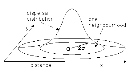
If this is true, dispersal distance can simply measured as the standard deviation, , of the dispersal distribution.  A population "neighbourhood" can be defined approximately as a group of individuals who come from an area 2 wide.

[Strictly,  is a valid measure of dispersal only if dispersal is exactly normally distributed. Many field studies have shown that dispersal is actually leptokurtic, i.e. most offspring breed very close to their parents, but some breed an enormous distance away. In practice, it doesn't much matter if dispersal is non-normal, provided it is not too extreme.]

Neighbourhood population size

The neighbourhood population size was defined by Wright as the population size in a within a neighourhood of radius 2 where population density is d.  Therefore, the neighbourhood population size, Nb = 4²d.  The neighbourhood population size plays the same role as the value of Nm in the island model: it determines the amount of variation between populations at equilibrium between gene flow and drift, measured by F_ST.  Like Nm, the neighbourhood size is a product of population number and migration rate.  But because the isolation by distance model is more realistic than the island model (at least, for most situations), it is potentially more useful.  For isolation by distance, we can estimate population density and dispersal distance, and estimate the value of neighbourhood size, and hence the expected levels of variation from population to population.  Many people try to apply the island model to spatially extended, continuous populations, but it wasn't really designed for such use.

So today we have covered simple ideas of subdivided populations, and shown how selection in a patchy environment may maintain polymorphisms, even with random mating. We then went on to discuss the evolutionary effects of migration (it homogenizes gene frequencies), discussed how differentiation produces an overall heterozygote deficit (F_ST) at the metapopulation level, even though there is random mating within subpopulations. If differentiation is caused by genetic drift in small local populations, then this F_ST measures a kind of inbreeding.

We then discussed how to use this measure to study the equilibrium between drift and migration. The former tends to cause differentiation, the latter to homogenize gene frequencies. This is a drift/migration balance, but you might also imagine situations where the differentiation is produced by patchy selection, producing a selection/migration balance. Geographic selection that is more consistent over larger areas is covered in more depth in Evolution in space and time.

FURTHER READING

FUTUYMA, DJ 1998. Evolutionary Biology.  Chapter 11 (pp. 314-329).