OLD! - For current see BIOSCIENCES COURSE SITE
BIOL2007 - INBREEDING AND NEUTRAL EVOLUTION
SO FAR,
we have dealt chiefly with deterministic evolution,
via natural selection.
TODAY,
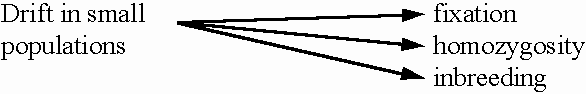
we explore the effects of finite population size and inbreeding on genetic
variation, and show that this can lead to random
evolutionary change (or "drift"). Mutation is, of course, a sort of random
genetic change, but genetic drift can work much faster.
 First
we must study the theory of inbreeding, which can be "regular", for instance
in sib-sib mating such as the Pharaohs of Ancient Egypt, or as a simple
effect of random mating in small populations. We first study regular
systems of inbreeding, then go on to how small population sizes
can cause both genetic drift and inbreeding.
First
we must study the theory of inbreeding, which can be "regular", for instance
in sib-sib mating such as the Pharaohs of Ancient Egypt, or as a simple
effect of random mating in small populations. We first study regular
systems of inbreeding, then go on to how small population sizes
can cause both genetic drift and inbreeding.
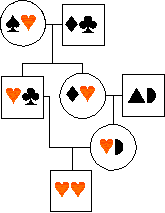
MEASURING INBREEDING
If an individual mates with a relative
(or with itself! as in some plants or snails), the offspring may be homozygous
for a copy of an allele which is identical by
descent from one of the ancestors:
... in the diagram, a male is homozygous
for two copies of an allele - -
inherited from a single copy in an ancestor. This is partly because his
mum was also his dad's niece (a type of inbreeding that is common in many
human societies).
-
inherited from a single copy in an ancestor. This is partly because his
mum was also his dad's niece (a type of inbreeding that is common in many
human societies).
The INBREEDING
COEFFICIENT, F, is used to gauge the strength
of inbreeding. F = probability that two alleles in an individual
are identical by descent (IBD).
F
stands for fixation index, because of the increase in homozygosity,
or fixation, that results from inbreeding.
Note: two alleles that are identical
by descent must be identical in state.
However, a homozygote for an identifiable allele can often be produced
without inbreeding in its recent ancestry. Thus identity
in state does not necessarily imply identity by descent.
Is inbreeding
always bad?
Inbreeding is not
generally recommended because of the existence of deleterious recessive
alleles in most populations. Although these should be rare per gene
(usually much less than 10-3, see mutation-selection
balance), there will be many deleterious alleles per genome.
According to some estimates, you and I each carry about 1 strongly deleterious
hidden mutation. When homozygous, these mutations reduce fitness; inbreeding
will therefore lead to inbreeding depression
as the homozygous mutations become expressed.
However, inbreeding
isn't all bad, and many organisms habitually inbreed. Animals such
as fig wasps and certain parasites regularly mate with their siblings,
and selfing is common in many of the most aggressive weeds of agriculture.
The advantage is presumably ecological, since a single female can then
colonize an empty resource or host. There may also be a genetic advantage
by preventing recombination between adaptive loci. One assumes deleterious
recessives in habitually inbreeding species have mostly been purged
by selection.
In human societies
where some families have a lot of wealth, or where a bridal dowry is paid,
inbreeding is common. Examples are European royal families, and on
the Indian subcontinent. Perhaps here the idea is to prevent the
"recombination" of wealth with other families!
In any case, mild
inbreeding, such as mating between first cousins, or uncle-niece isn't
so dangerous. Charles Darwin married his first cousin, Emma Wedgewood,
and had an astonishing 10 children. Some were sickly or died young,
but this was common in the days before penicillin.
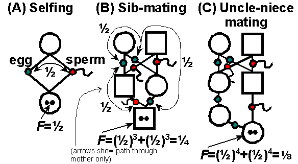
REGULAR SYSTEMS
OF INBREEDING
We can measure F easily in
regular systems of inbreeding, using Sewall Wright's method of "path analysis":
1) Find each path that alleles
may take to become IBD.
2) Find the number of path segments (x)
between gametes (eggs or sperm) through a single ancestor in common in
each path.
3) Calculate the probability of IBD
for each path. The probability that an allele is IBD between two
gametes connected through an individual is 1/2. Thus, the probability
of IBD for each path is (1/2)x.
4) Add up the probabilities of each path
to get the total probability of IBD.
Calculations like these are used in genetic
counselling, and in animal breeding and in zoos to avoid inbreeding depression.
Some examples:
 EFFECT
OF INBREEDING ON POPULATIONS
EFFECT
OF INBREEDING ON POPULATIONS
Consider two alleles, A, and a
with frequencies p,q with inbreeding (IBD) at rate F:
Frequency of homozygotes:
AA = (1-F)p2
[outbred] + Fp[inbred]
(see figure at right)
= p2 + F(p-p2)
= p2 + Fp(1-p)
= p2 + Fpq
Similarly the frequency of the other homozygotes,
aa=
q2
+
Fpq
All genotype frequencies must add to 1,
so the extra 2Fpq AA
and aa
homozygotes must have come from the heterozygotes (which cannot be IBD,
since they arent even identical in state), and so overall, the frequencies
are:
genotype       AA        Aa       aa
frequency    p2+Fpq   2pq(1-F)  q2+Fpq   Sum = 1
So, inbreeding
leads to a reduction in heterozygosity
within the population. The heterozygosity
(Het, i.e. the proportion that are heterozygotes under inbreeding)
is reduced by a fraction
F compared with the outbred (Hardy-Weinberg)
expectation HetHW = 2pq:
Het
= HetHW (1 - F)
Therefore, as well as measuring a probability
(of IBD), F also measures reduction of heterozygosity,
or heterozygote deficit
compared to Hardy-Weinberg. The heterozygote deficit = the level of inbreeding
(in the absence of selection, assortative mating, migration, etc.).
GENETIC DRIFT
Deterministic
vs. stochastic evolution
The Hardy-Weinberg
law is the basis of all population genetics theory, but it assumes that
in the absence of selection or other evolutionary forces, absolutely no
gene frequency change occurs during reproduction. This would be true
in an infinitely large population; under these conditions, selection would
be completely predictable and deterministic.
However, this is
only approximately true in real populations of finite size. Assume
a diploid population of constant size N. Each of 2N
alleles are copied into gametes, which unite to form the next generation.
Even if the alleles are equal in fitness (neutral), some will not reproduce,
while others will manage to transmit several copies to the next generation.
Below is an example
of drift. Imagine a rare species kept in a zoo with a population of only
six diploid individuals. There are a total of 12 alleles (numbered 1-12
in generation 0). All alleles are assumed equally fit, so that evolution
is neutral. The alleles may also be genetically distinguishable, or "different
in state" (represented by colours).
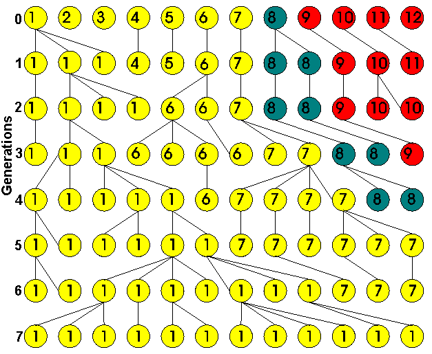
If the wild source population were large,
all the alleles in generation 0 would have come from different ancestors;
none would be identical by descent (IBD).
However, by chance some alleles are lost in each generation. After a moderate
number of generations, every allele will ultimately become a copy of just
one of the original alleles, or IBD.
In
the diagram, all the alleles happen to become IBD to allele 1 by
the 7th generation. Another way of saying this is that, looking backwards
in time, the coalescence time
of the alleles in the final population is 7 generations ago.
Alleles that are
IBD
must also be identical in state
(barring mutation). Because the population has become fixed for allele
1, it has also become fixed for the allelic state to which allele 1 belongs
("yellow"). Usually, there are fewer allelic states than alleles,
so that fixation of state (gen. 5, above) can happen earlier than identity
by descent (gen. 7). Random evolution in frequency of allelic states
is called genetic drift.
This kind of evolution
is not predictable; it is random or stochastic.
Stochastic evolution occurs in any finite population, whether or not selection
is operating -
no evolution is completely deterministic.
Even in large populations, evolution is only approximately deterministic.
Drift is slower in
larger populations. Why? If I tossed a coin twice, and get 2 heads,
you would not be surprised. If I tossed 20 times, and got 20 heads
you would be very surprised. If I scored 200 heads in as many tosses,
you would rightly suspect me of cheating. Similarly, if we have two
alleles in a population (equivalent to heads and tails), we get a larger
variance of allele frequency if we have a small population. This is equivalent
to getting a more variable fraction of heads when tossing a coin a small
number of times.
Predictable
unpredictability (remember, science
= accurate prediction!)
We can't predict
exactly
what is going to happen in genetic drift, but the distribution of
results is known, and useful. We can quantify the following:
1) The mean
gene frequency. The probabilities for
two alleles in a single generation are given by the binomial distribution,
with binomial probability p and numbers of trials
n.
The mean, or expected frequency
in the future is simply the binomial probability p (similarly,
the average fraction of heads is 0.5; the same as the probability of a
single head on each throw).
2) The variance
of gene frequency after one generation.
The binomial variance is:
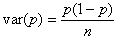
The standard
deviation (SD)
of allele frequency is a good measure of the speed of genetic drift (remember,
the mean stays the same). The SD is the square root of the variance;
here, if N is the population size of a diploid population,
then the total number of alleles, (n in the binomial
formula), is 2N, so the standard deviation of allele
frequency after one generation is:

So supposing we are
interested in the rate of drift of the yellow allele which has initial
frequency 0.583 in the diagram above. In a population with 2N
= 12 alleles, the SD of allele frequency in a single generation will be
0.142; this contrasts with 0.049 for 2N = 100, and 0.016
for 2N = 1000. The 95% confidence limits of the gene
frequency after a single throw can be calculated approximately, given that
the binomial has an approximately normal distribution, as +/- 2 S.D.s from
the mean.
Knowing the
variance for a single generation, we can predict the long-term consequences
of drift, including the probability distribution for allele frequency after
a given number of generations. (The maths is, unfortunately, beyond this
course!).
3) The probability
that a particular allele will eventually be fixed.
We know that one of the alleles will eventually take over; the probability
that it will be any particular allele is simply the fraction that the allele
has in the population initially, or  .
.
4) Eventually, any
population will become fixed for one of the original alleles, and we can
also predict approximately how long this will take. Looking backwards,
this is the coalescence time
of a given population. The coalescence time is given by (rate of fixation)-1
(see below) and will therefore be about 2N generations.
 EXAMPLES
OF GENETIC DRIFT
EXAMPLES
OF GENETIC DRIFT
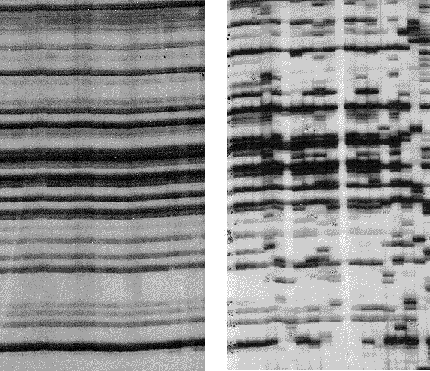
Genetic drift is important in nature.
Here is a recent example from an Asian bramble (Rubus alceifolius)
which is an introduced weed on some Pacific islands. Genetic variation
was studied by means of a DNA fingerprint technique called "Amplified Fragment
Length Polymorphisms" - AFLP for short. Each vertical "lane" on the
gel represents DNA from a single individual; each AFLP band is thought
to represent an independent DNA fragment, and polymorphisms are revealed
by presence or absence of bands. In its native range (Vietnam, right),
this species is highly polymorphic, while in an introduced population (the
island of Réunion, left), no polymorphisms are observed. This suggests
that the founder population was very small, and that all variation has
been lost. (see Amsellem L et al. 2000.Mol. Ecol.
9: 443-455, reproduced by permission).
GENETIC DRIFT
AS A CAUSE OF INBREEDING
As we have seen, inbreeding
results from drift because alleles become identical
by descent (IBD). We can therefore measure drift in terms
of our inbreeding coefficient, F:
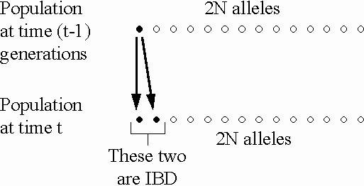
In a population of size N, the
probability that two alleles picked during random mating
in generation t are IBD
due to copying from generation t-1
is  (on average).
This is the rate of inbreeding
due to drift per generation.
(on average).
This is the rate of inbreeding
due to drift per generation.
BUT the 2N alleles in the
previous generation may be IBD themselves from inbreeding in previous
generations. The fraction of alleles in generation
t that
are IBD because of inbreeding before generation t-1
is:
Summing the inbreeding from previous generations
together with inbreeding leading to the current generation at time t,
we have:
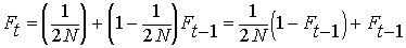
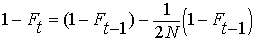
By definition, the heterozygosity after a
single generation of inbreeding, Het = HetHW
(1 - F). (See above under EFFECT
OF INBREEDING ON POPULATIONS).
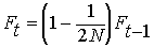
From the above equation relating Ft to
Ft-1,
and cancelling the HetHW (HetHW
= 2pq remains the same between generations, because the expected
gene frequency p remains the same, but the actual Het will
change):
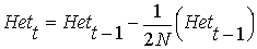
rearranging ...
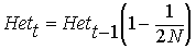
therefore, after t generations
of drift:
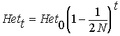
Thus, heterozygosity
declines approximately by a factor
per generation. However, ...
(a) This is true only on
average because a single allele may have zero, one, two or more
copies in the next generation. The factor
is an average for each allele.
(b) F can also measure inbreeding
as a result of subdivision into two or more finite populations. Remember
that when we assumed Hardy-Weinberg, we also assumed a lack of migration
(i.e. mixing of populations).
When we sample from a number of sub-populations
with different gene frequencies which do not mate randomly with each other,
the heterozygote deficit gives us a measure of identity by descent produced
by the population subdivision.
This between-population inbreeding is usually
written FST, meaning
inbreeding (F) due to
subdivision into Subpopulations
relative to the Total population.
For example, assume many populations of
finite size N start from from the same gene frequency and
drift apart for t generations. Within
each randomly mating population there is no heterozygote deficit,
of course, but each population is accumulating identity by descent at a
rate of
per generation (on average). Between populations,
this results in an increasing heterozygote deficit, or deviation from Hardy-Weinberg.
This heterozygote deficit is measured
by FST. If all populations
are of size N, the FST should
be equal to the level of identity by descent or
inbreeding, F, produced on average by drift within
each population relative to the initial source population. Neat,
eh?!
You can try some simulations of drift yourself;
go to natural
selection and drift simulations. You can use some of these (DRIFT.EXE,
and PDRIFT.EXE) to get an estimate of the level of inbreeding and heterozygote
deficit (F or FST) accumulated during
genetic drift of up to 100 populations.
FST
is widely used to study gene frequency variation over a geographic range
as a measure of population subdivision. This topic, which we can't
cover here (shame!), is often referred to as population
structure.
EFFECTIVE POPULATION
SIZE
Even with no deterministic
bias, or natural selection, alleles usually do not have identical probability
of being passed on, as required in these simple models. Population
geneticists get around this by calculating an idealized, or effective
population size that produces approximately
the same rate of genetic drift in their simple models as does the actual
population with all its complexity. The effective population size
may be rather different from the actual population size. Two examples:
1) Separate
sexes. The simple theory above assumes that a single individual may
have two alleles IBD for a single allele in the previous generation.
In fact, they can only do this if there is selfing. In dioecious
organisms like us, this is not (yet!) possible. Separate sexes therefore
enforce some outbreeding, and slow the buildup of identity by descent:
the effective size is marginally larger than the actual population size.
2) Unequal sex ratio.
In species which maintain harems, like the elephant seal (see later in
SEX
AND SEXUAL SELECTION), a single
male may commandeer almost all the matings by fighting off other males.
Similarly, in modern cow herds almost all females are fertilized artificially;
a single bull provides enough sperm for thousands of offspring. Although
there are millions of cows in Britain, calves are mostly progeny of very
few bulls. The effective population size may therefore be in the hundreds
rather than millions, because genes in the population are funnelled through
these few bulls in every generation.
FINALE
During this lecture, we measured inbreeding
using the inbreeding coefficient,
F.
We applied this method to
regular systems of inbreeding,
and then tried something a bit trickier: to use F to measure
inbreeding
due to genetic drift in finite populations.
The Hardy-Weinberg law is very useful,
and simple models of natural selection work well most of the time. However,
these models have the ever-so-slight drawback that they depend on an assumption
of infinite population sizes. Before today, we modeled evolution in terms
of infinitely divisible gene frequencies. In fact this is simply doesn't
work: some of the most interesting evolution happens when we mix random
genetic drift -- due to finite population sizes -- with deterministic
forces -- selection. Drift may or, may not be important in evolution, but
it always happens, because populations are always finite.
For now, it is worth knowing that the equation
characterizes perhaps the most important genetic problem in conservation.
The equation will be important in any species with low overall N;
for instance in many endangered large mammals, such as tigers in the Gir
forest in India, Florida panthers, and Sumatran rhinos.
Well! That's probably enough for
today!
FURTHER READING
FUTUYMA, DJ 1998.
Evolutionary Biology. Chapter 11 (pp. 297-314).
Population
Structure lecture notes (optional!).
Back to BIOL
2007 TIMETABLE