MATH0043 §2: Calculus of Variations |
Contents
What is the Calculus of Variations?
Many problems involve finding a function that maximizes or minimizes an
integral expression.
One example is finding the curve giving the
shortest distance between two
points — a straight line, of course, in Cartesian geometry (but can you prove
it?) but less obvious if the two points lie on a curved
surface (the problem of finding geodesics.)
The mathematical techniques developed to solve this type of problem
are collectively known as the calculus of variations.
1 Functionals and Extrema
Typical Problem: Consider a definite integral that depends on an unknown function y(x), as
well as its derivative y′(x)=d y/d x,
A typical problem in the calculus of variations involve finding a particular
function y(x) to maximize or minimize
the integral I(y) subject to boundary conditions y(a)=A and
y(b)=B.
Definition 1
The integral I(y) is an example of a functional, which (more
generally) is a mapping from a set of allowable functions to the
reals.
We say that I(y) has an extremum when I(y) takes its maximum or minimum value.
2 The Statement of an Example Problem
Consider the problem of finding the curve y(x) of shortest length that
connects the two points (0,0) and (1,1) in the plane. Letting ds be an element of arc length, the arc
length of a curve y(x) from x=0 to x=1 is ∫01 ds. We can
use Pythagoras’ theorem to relate ds to dx and dy: drawing a
triangle with sides of length dx and dy at right angles to one
another, the hypotenuse is ≈ ds and so ds2 = dx2 + dy2 and
s = √dx2 + dy2 = √1+
(dy/dx)2 dx. This means the arc length equals
∫01 √1+y′2 dx.
The curve y(x) we are looking for minimizes the functional
| I(y)=
| ∫ | | ds = | ∫ | | (1+(y′)2)1/2 dx subject
to boundary conditions y(0)=0, y(1)=1 |
which means that I(y) has an extremum at y(x).
It seems obvious that the solution is y(x)=x, the straight line
joining (0,0) and (1,1), but how do we prove this?
3 The Euler-Lagrange Equation, or Euler’s Equation
Definition 2 Let Ck[a,b] denote the set of continuous
functions defined on the interval a ≤ x ≤ b which have their first
k-derivatives also continuous on a ≤ x ≤ b.
The proof to follow requires the
integrand F(x,y,y′) to be twice differentiable with respect to each
argument. What’s more, the methods that we use in this module to solve
problems in the calculus of variations will only find those solutions
which are in C2[a,b]. More advanced
techniques (i.e. beyond MATH0043)
are designed to overcome this last restriction. This isn’t just a
technicality: discontinuous
extremal functions are very important in optimal control problems, which
arise in engineering applications.
Theorem 1
If I(
Y)
is an extremum of the functional
defined on all functions y ∈
C2[
a,
b]
such that y(
a)=
A,
y(
b)=
B, then Y(
x)
satisfies the second order ordinary
differential equation
| | | ⎛
⎜
⎜
⎝ | | | ⎞
⎟
⎟
⎠ | −
| | = 0. (1) |
Definition 3 Equation (1) is the
Euler-Lagrange equation, or sometimes just Euler’s
equation
. Warning 1
You might be wondering what ∂
F/∂
y′
is suppose
to mean: how can we differentiate with respect to a derivative? Think
of it like this: F is given to you as a function of three variables,
say F(
u,
v,
w)
, and when we evaluate the functional I we plug in x,
y(
x),
y′(
x)
for u,
v,
w and then integrate. The derivative ∂
F/∂
y′
is just the partial derivative of F with respect to its second
variable v. In other words, to find ∂
F/∂
y′
,
just pretend
y′ is a variable
.Equally, there’s an important difference between d F/d x and
∂ F/∂ x. The former is the derivative of F
with respect to x, taking into account the fact that y= y(x) and
y′= y′(x) are functions of x too. The latter is the partial
derivative of F with respect to its first variable, so it’s found by
differentiating F with respect to x and pretending that y and y′
are just variables and do not depend on x. Hopefully the next example
makes this clear:
Example 1 Let F(
x,
y,
y′) = 2
x +
xyy′ +
y′
2 +
y. Then
|
| | = xy + 2y′ | | | | | | | | | |
| = y + xy′ + 2y′′ | | | | | | | | | |
| = xy′ + 1 | | | | | | | | | |
| = 2+yy′ | | | | | | | | | |
| = 2 + y y′
+ xy′ 2
+ xyy′ ′ + 2y′′
y′ + y′
| | | | | | | | | |
|
and the
Euler–Lagrange equation is
Warning 2 Y satisfying the Euler–Lagrange equation is a necessary, but not
sufficient, condition for I(Y) to be an extremum. In other
words, a function Y(x) may satisfy the Euler–Lagrange equation even
when I(Y) is not an extremum.
Proof.
Consider functions Yє(x) of
the form
where η(x)∈ C2[a,b] satisfies
η(a)=η(b)=0, so that Yє(a)=A and Yє(b)=B,
i.e. Yє still
satisfies the boundary conditions. Informally, Yє is a
function which satisfies our boundary conditions and which is ‘near to’
Y when є is small.1
I(Yє) depends on the value of є, and we write
I[є] for the value of I(Yє):
When є = 0, the function I[є] has an extremum and so
We can compute the derivative dI/dє by differentiating
under the integral sign:
| = | | | ∫ | | F(x,Yє,
Yє′) dx = | ∫ | | | | (x,Yє,
Yє′) dx |
We now use the multivariable chain rule to differentiate F with
respect to є. For a general three-variable function F(u(є),
v(є),w(є)) whose three arguments depend on є,
the chain rule tells us that
In our case, the first argument x is independent of є, so
d x/d є= 0, and since Yє= Y+є η we
have d Yє/d є = η and
d Yє′/d є = η′. Therefore
| (x,Yє,Yє′) = | | η(x) + | | η′(x). |
Recall that d I/d є=0 when є = 0. Since Y0 =
Y and Y0′ = Y′,
|
0 = | ∫ | | | | (x,Y,Y′) η(x) +
| | (x,Y,Y′)η′(x) d x.
(2) |
Integrating the second term in (2) by parts
| ∫ | | | | η′(x) dx = | ⎡
⎢
⎢
⎣ | | η(x) | ⎤
⎥
⎥
⎦ | | −
| ∫ | | | | | ⎛
⎜
⎜
⎝ | | | ⎞
⎟
⎟
⎠ | η(x) dx. |
The first term on the right hand side vanishes because
η(a)=η(b)=0.
Substituting the second term into (2),
| ∫ | | | ⎛
⎜
⎜
⎝ | | − | |
| | ⎞
⎟
⎟
⎠ | η(x) dx = 0. |
The equation above holds for any η(x)∈ C2[a,b] satisfying
η(a)=η(b)=0, so the fundamental
lemma of calculus of variations (explained on the next page) tells us
that Y(x) satisfies
Definition 4
A solution of the Euler-Lagrange equation is called an
extremal
of the functional.2
Exercise 1 Find an extremal y(
x)
of the functional
| I(y)= | ∫ | | (y′−y)2 dx, y(0)=0, y(1)=2, | ⎡
⎢
⎢
⎣ | Answer:
y(x)=2 | | | ⎤
⎥
⎥
⎦ | . |
Exercise 2 By considering y+g, where y is the solution from
exercise 1 and g(x) is a variation in
y(x) satisfying g(0)=g(1)=0, and then considering I(y+g), show explicitly
that y(x) minimizes I(y) in Exercise 1 above.
(Hint: use integration by parts, and the
Euler–Lagrange equation satisfied by y(x) to simplify the expression for
I(y+g)).
Exercise 3 Prove that the straight line y=x is the curve giving the
shortest distance between the points (0,0) and (1,1).
Exercise 4 Find an extremal function of
| I[y]= | ∫ | | x2(y′)2+y dx, y(1)=1, y(2)=1, | ⎡
⎢
⎢
⎣ | Answer:
y(x)= | | lnx+ | | +1−ln2 | ⎤
⎥
⎥
⎦ | .
|
MATH0043 Handout: Fundamental lemma of the calculus of variations
In the proof of the Euler-Lagrange equation, the final step invokes a lemma
known as the fundamental lemma of the calculus of
variations (FLCV).
Lemma 1 (FLCV). Let y(
x)
be continuous on [
a,
b]
, and suppose that for all
η(
x) ∈
C2[
a,
b]
such that η(
a)=η(
b)=0
we have
Then y(
x)=0
for all a ≤
x ≤
b. Here is a sketch of the proof. Suppose, for a contradiction, that for
some a < α < b we have y(α)>0 (the case when α=a or
α = b can be done similarly, but let’s keep it simple). Because y is
continuous, y(x)>0 for all x in some interval (α0, α1)
containing α.
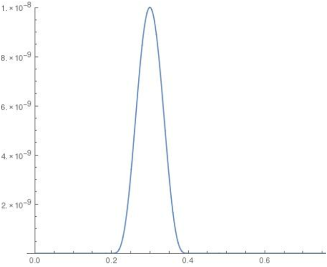
Consider the function η : [a,b] → ℝ defined by
|
η(x) = | ⎧
⎨
⎩ | | (x−α0)4 (x−α1)4 | α0 < x < α1 |
| 0 | otherwise.
|
|
|
η is in C2[a,b] — it’s difficult to give a formal proof
without using a formal definition of continuity and differentiability,
but hopefully the following plot shows what is going on:
| Figure 1: The function η defined above, if a=0, b=1,
α0=0.2, α1 = 0.4. |
By hypothesis, ∫01 y(x)η(x) dx = 0. But y(x)η(x) is
continuous, zero outside (α0, α1), and strictly positive
for all x ∈ (α0, α1). A strictly positive continuous
function on an interval like this has a strictly positive integral, so
this is a contradiction. Similarly we can show y(x) never takes
values <0, so it is zero everywhere on [a,b].
4 The Brachistochrone
A classic example of the calculus of variations is to find
the brachistochrone, defined as that smooth curve joining two
points A and B (not underneath one another) along which a particle will
slide from A to B under gravity in the fastest possible time.
Using
the coordinate system illustrated,
we can use conservation of energy to obtain the velocity v of the particle
as it makes its descent
so that
Noting also that distance s along the curve s satisfies ds2=dx2+dy2, we
can express the time T(y) taken for the particle to descend along the
curve y=y(x) as a functional:
| T(y)= | ∫ | | dt = | ∫ | | | | = | ∫ | | | | =
| ∫ | | | | dx, subject
to y(0)=0, y(h)=a. |
The brachistochrone is an extremal of this functional,
and so it satisfies the Euler-Lagrange equation
| | ⎛
⎜
⎜
⎜
⎜
⎝ | | | ⎞
⎟
⎟
⎟
⎟
⎠ | =0, y(0)=0, y(h)=a. |
Integrating this, we get
where c is a constant,
and rearranging
We can integrate this equation using the substitution
x=α sin2θ to obtain
| y= | ∫ | | | dx= | ∫ |
| | 2 α sinθ cosθ
dθ = | ∫ | α (1−cos2θ) dθ =
| | (2θ−sin2θ)+k. |
Substituting back for x, and using y(0)=0 to set k=0, we obtain
Definition 5 This curve is called a cycloid.
The constant α is determined implicitly by the remaining boundary
condition y(h)=a.
The equation of the cycloid is often given in the following parametric form (which can
be obtained from the substitution in the integral)
and can be constructed by following the locus of the initial point of
contact when a circle of radius α/2 is rolled (an angle 2θ)
along a straight line.
5 Functionals leading to special cases
When the integrand F of the functional in our typical calculus of
variations problem does not depend explicitly on x, for example if
extremals satisfy an equation called the Beltrami identity which
can be easier to solve than the Euler–Lagrange equation.
Theorem 2
If I(
Y)
is an extremum of the functional
defined on all functions y ∈
C2[
a,
b]
such that y(
a)=
A,
y(
b)=
B
then Y(
x)
satisfies
for some constant C. Definition 6
(3) is called the Beltrami identity or Beltrami
equation. Proof.
Consider
| | | ⎛
⎜
⎜
⎝ | F− y′ | |
| ⎞
⎟
⎟
⎠ |
= | | −y′′ | | −y′ | |
| ⎛
⎜
⎜
⎝ | | | ⎞
⎟
⎟
⎠ | . (4) |
Using the chain rule to find the x-derivative of F(y(x),y′(x))
gives
so that (4) is equal to
| y′ | | + y′′ | |
− y′ ′ | | − y′ | | | |
= y′ | ⎛
⎜
⎜
⎝ | | − | | | | | ⎞
⎟
⎟
⎠ |
Since Y is an extremal, it is a solution of the Euler–Lagrange
equation and so this is zero for y=Y. If something has zero
derivative it is a constant, so Y is a solution of
for some constant C.
Exercise 5 (Exercise 1 revisited): Use the Beltrami identity to find
an extremal of
| I(y)= | ∫ | | (y′−y)2 dx, y(0)=0, y(1)=2, |
Answer:
(again).
6 Isoperimetric Problems
So far we have dealt with boundary conditions of the form
y(a)=A,y(b)=B or y(a)=A, y′(b)=B. For some problems the natural
boundary conditions are expressed using an integral. The standard
example is
Dido’s
problem3: if you have a piece of rope with a
fixed length, what shape should you make with it in order to enclose the
largest possible area? Here we are trying to choose a function y
to maximise an integral I(y) giving the area enclosed by y, but the
fixed length constraint is also expressed in terms of an integral
involving y. This kind of problem, where we seek an extremal of some
function subject to ‘ordinary’ boundary conditions and also an integral
constraint, is called an isoperimetric problem.
A typical isoperimetric problem is to find an
extremum of
| I(y)= | ∫ | | F(x,y,y′) dx, subject to y(a)=A, y(b)=B,
J(y)= | ∫ | | G(x,y,y′) dx=L. |
The condition J(y)=L is called the integral constraint.
Theorem 3
In the notation above, if I(
Y)
is an extremum of I subject to
J(
y)=
L, then Y is an
extremal of
| K(y)= | ∫ | | F(x,y,y′)+ λ G(x,y,y′) dx
|
for some constant λ
.
You will need to know about
Lagrange
multipliers to understand this
proof: see the handout on moodle (the constant λ will turn out
to be a Lagrange multiplier).
Proof.
Suppose I(Y) is a maximum or minimum subject to J(y)=L, and
consider the two-parameter family of functions given by
where є and δ are constants and
η(x) and ζ(x) are
twice differentiable functions such that
η(a)=ζ(a)=η(b)=ζ(b)=0, with ζ chosen so that
Y+є η + δ ζ obeys the integral constraint.
Consider the functions of two variables
| I[є, δ] = | ∫ | | F(x,Y+є η +
δ ζ,Y′+є η′ +δ ζ′) dx,
J[є, δ] = | ∫ | | G(x,Y+є η +
δ ζ,Y′+є η′ +δ ζ′) dx.
|
Because I has a maximum or minimum at Y(x) subject to J=L,
at the point (є,δ)=(0,0) our function
I[є, δ] takes an extreme
value subject to J[є, δ]=L.
It follows from the theory of Lagrange multipliers that
a necessary condition for a function I[є, δ] of two variables
subject to a constraint J[є, δ]=L
to take an extreme value at (0,0) is that there is a constant
λ (called the Lagrange multiplier) such that
at the point є = δ = 0.
Calculating the є derivative,
| = | | ∫ | | | | | ⎛
⎝ | F(x,Y+є η + δ ζ,Y′+є η′ +δ
ζ′) +λ G(x,Y+є η + δ ζ,Y′+є η′ +δ
ζ′) | ⎞
⎠ | dx |
|
| | = | | ∫ | | η | | ⎛
⎝ | F+λ G | ⎞
⎠ | + η′
| | | ⎛
⎝ | F+λ G | ⎞
⎠ | dx (chain
rule) |
|
| | = | | ∫ | | η | ⎛
⎜
⎜
⎝ | | ⎛
⎝ | F+λ G | ⎞
⎠ | −
| | | ⎛
⎜
⎜
⎝ | | | ⎛
⎝ | F+λ G | ⎞
⎠ |
| ⎞
⎟
⎟
⎠ | ⎞
⎟
⎟
⎠ | dx (integration by parts) |
|
| | | |
| | = | 0 when є=δ=0, no matter what η is.
|
|
Since this holds for any η, by the FLCV (Lemma 1) we get
| (Fy + λ Gy) ( x,Y,Y′) + | | (Fy′ + λ Gy′)
(x,Y,Y′) = 0 |
which says that Y is a solution of the Euler–Lagrange equation for
K, as required.
Note that to complete the solution of the problem, the initially unknown
multiplier λ must be determined at the end using the constraint
J(y)=L.
Exercise 6 Find an extremal of the functional
| I(y) = | ∫ | | (y′)2 dx, y(0)=y(1)=1, |
subject to the constraint that
| J(y)= | ∫ | | y dx=2. | ⎡
⎢
⎢
⎢
⎢
⎢
⎣ |
Answer: y=f(x)=−6 | ⎛
⎜
⎜
⎝ | x− | | ⎞
⎟
⎟
⎠ | | + | | . | ⎤
⎥
⎥
⎥
⎥
⎥
⎦ |
Exercise 7 (Sheep pen design problem): A fence of length l must be
attached to a straight wall at points A and B (a distance a apart, where
a<l) to form an enclosure. Show that the shape of the fence that maximizes
the area enclosed is the arc of a circle, and write down (but do not try to
solve) the equations that determine the circle’s radius and the location of
its centre in terms of a and l.
Suggested reading
There are many introductory textbooks on the calculus of variations, but
most of them go into far more mathematical detail that is required for
MATH0043. If you’d like to know more of the theory, Gelfand and Fomin’s
Calculus of Variations is available in the library. A less
technical source is chapter 9 of Boas Mathematical Methods in the
Physical Sciences. There are many short introductions to calculus of
variations on the web, e.g.
although all go into far more detail than we need in MATH0043. Lastly,
as well as the moodle handout you may find
useful as a refresher on Lagrange multipliers.
This document was translated from LATEX by
HEVEA.