Elasticity and Equations of State

The way planets deform depends primarily upon the elastic properties of the constituent polycrystalline materials. In particular, the speed of body waves passing through a material is entirely dependant upon the ratio of the elastic modulus of that material to its density. Whenever any external force is applied to a system, there is a resultant strain; similarly, whenever a system is strained in some way, there is then some stress upon the system. For example, squashing a jelly will deform it; deforming a jelly will result in a restoring force or stress eager to return the jelly to its original shape.

Stress, Strain and Elastic Moduli:

An elastic modulus is just the ratio of stress to the associated strain. We wish to understand only the basic elastic equations and the physical meaning of these equations.

For a stress, σ (hydrostatic, shear, axial...), resulting in an elastic deformation strain, ε:

σ = Mε

where M is an elastic modulus (bulk, shear, Young's...).

For a hydrostatic stress (i.e., equally applied forces in all directions), which is often assumed within planetary interiors, the stress is the hydrostatic pressure:

σ = ΔP

and the strain is the relative change in volume of the system:

ε = -ΔV/V

therefore:

ΔP = -M(ΔV/V)

and the elastic modulus in this case is the incompressibility or bulk modulus:

M = -V(ΔP/ΔV) = K

Stress, Strain, and Tensors:

The stress, σ, does not have to be hydrostatic; there may be unequally applied stresses in all directions, and therefore the stress is tensorial: 

And can be represented thus:

where σ_ij is the stress acting in the x_i direction on the plane perpendicular to the x_j direction; σ_i=j are the axial stresses and σ_i≠j are the shear stresses.

The strain ε_ij is also a second order tensor.

Therefore the elastic moduli, or elastic constants, are fourth order tensors:

The stress, σ, and the strain, ε, must be symmetric, and the nature of c_ijkl depends on the symmetry of the crystal. It is customary to use a contracted notation thus:

c₁₁₁₁ → c₁₁ elastic constant relations σ₁₁ to ε₁₁

c₁₁₂₂ → c₁₂ elastic constant relations σ₁₁ to ε₂₂

c₂₃₂₃ → c₄₄ elastic constant relations σ₂₃ to ε₂₃

In general, 11→1; 22→2; 33→3; 23=32→4; 13=31→5; 12=21→6.
 
 

Cubic crystals:

There are a maximum of 21 elastic constants for a crystalline body, but for cubic crystals the elastic constants, c_ij, may be reduced to just three independent elastic constants:

c₁₁= c₂₂ = c₃₃ → modulus for axial compression, i.e., a stress σ₁₁ results in a strain ε₁₁ along an axis;

c₄₄ = c₅₅ = c₆₆ → shear modulus, i.e., a shear stress σ₂₃ results in a shear strain ε₂₃ across a face;

c₁₂ = c₁₃ = c₂₃ → modulus for dilation on compression, i.e., an axial stress σ₁₁ results in a strain ε₂₂ along a perpendicular axis.

All other c_ij = 0.

For single crystals, the elastic constants can be related to common elastic moduli such as:

Shear modulus:

μ = c₄₄ and μ = (c₁₁- c₁₂)/2

Bulk modulus:

 K = (c₁₁+ 2c₁₂)/3

Polycrystalline aggregates:

In the simplest case, we can consider a polycrystalline aggregate of crystals in random orientations, which is therefore isotropic. For such an isotropic system, the elastic constants may be reduced to just two, called the Lamé Constants, which are a combination of those described above.

The estimation of the bulk properties from the elastic constants is fairly straightforward; however, when dealing with real materials, e.g., rocks, which are made up of polycrystalline aggregates, the elastic properties have to be evaluated by averaging the elastic constants over all the crytalline structures within the aggregate. For polycrystalline materials made up of non-cubic crystals with lower symmetry, appropriate substitutions have to be made in the elastic constants to account for the asymmetry, e.g., <c₁₁>= (c₁₁+c₂₂+c₃₃), etc.. Therefore the bulk modulus becomes:

Elasticity and Seismic Velocity:

From an analysis of the passage of waves through a solid medium, the speed of seismic waves are given by:

Therefore, a knowledge of V_P and V_S is all that is required to obtain quantitative values for many elastic properties, some of which are outlined below.

Poisson's Ratio:

For uniaxial dilation (σ₁₁≠ 0; σ₂₂ = σ₃₃ = 0), Poisson's ratio is defined:

i.e., the ratio of thinning to elongation along perpendicular axes.

Analysis of the elastic constants gives Poisson's ratio in terms of more readily available parameters:

From this we can see that for an incompressible solid (K = ∞) or liquid (μ = 0), ν = 0.5; for an infinitely compressible solid (K = 0), ν = -1; thus we always have -1 < ν < 0.5, and generally ν ~ 0.25.

The seismic parameter:  

 Another useful quantity is the seismic parameter, which is defined by:

The Adams-Williamson equation:

If we recall that K = -VdP/dV = ρdP/dρ (since V/dV = -ρ/dρ ), then:

i.e. the seismic parameter gives a direct measure of density variation with depth.

However, at depth in the Earth, the pressure increases via:

ΔP = ρgΔr

so in the limit of ΔP, Δr → 0:

When combined with Φ = dP/dρ, this gives:

so the variation of density with depth can be inferred from the seismic parameter, and therefore from seismic velocities.

This is the Adams-Williamson Equation.

----------------------------------------------------------------------------------------------------------------------------

 
 Equations of State

An equation of state, EOS, describes how the volume, V, or density ρ, of a material system varies as a function of pressure, P, and temperature, T; it therefore allows us to determine a mineral composition (ρ or V) at depth (P and T).

In its simplest form, the EOS for an ideal gas may be given by:

PV=RT

where R is a constant, the gas constant; R = 8.31451 J K^-1 mol^-1. In other words, for a volume of ideal gas, V, experiencing an external pressure, P, there will be an associated increase in temperature of the gas given by PV/R.

More complex EOS are vital to planetary scientists, because in order to interpret seismic data to give Earth structure, or to rationalise planetary densities from moments of inertia and mass data, it is necessary to either:

(a) "compress and heat" mineral data to the PT state of a planetary interior, or

(b) "decompress and cool" planetary data to ambient conditions.

The simplest isothermal EOS for a solid is just the definition for incompressibility, or bulk modulus, K:

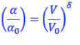
The simplest isobaric EOS for a solid is just the definition for the thermal expansion coefficient, α:

Although thermal expansion also changes with pressure via:

Where δ is approximately constant and is called the Anderson-Grüneisen parameter.

For most materials, the effect of pressure within planetary interiors is far greater than that of temperature; it is therefore easier to consider initially an isothermal EOS and then add on a thermal expansion correction. To this end, we shall first concentrate only on the effect of pressure, i.e., isothermal equations of state.

Isothermal Equations of State

We shall consider two types of isothermal EOS: infinitesimal EOS and finite strain EOS. The first treats volume expansion in terms of infinitesimally increasing increments in V, i.e., integrating over a volume or pressure range; the second treats volume expansion in term of finite differences in strain, i.e., considering the subsequent volume change as the original volume plus a little bit. Although the mathematics gets a bit tricky, especially for finite strain theory, the essential points of both methods are outlined below.

Infinitesimal Equations of State:

Isothermal EOS begin in their simplest form with the incompressibility, K. If we assume K is a constant (which is only true for small P), then integration of the definition for K gives:

where K₀ = K (0,T) is the incompressibility at P=0, T=constant.

However, if K was a constant, remaining unchanged with increasing pressure, then as P → ∞, ρ → ∞, which we know is impossible; indeed, both seismology and atomistic analysis show us that K increases with P, i.e., dK / dP > 0. In other words, the more you squash something, the harder it is to squash. At an atomic level, the more squashed a material becomes, the larger the repulsive forces become to resist the pressure, pushing the atoms apart.

If K is not a constant, we can repeat the whole integration process again, but at the next level of approximation, with:

K=K₀+K’P

i.e., K increases linearly with pressure. After integration, this gives: or,

This is the Murnaghan Integrated Linear Equation of State, MILEOS.

However, this equation is also still approximate since K' itself is also a function of P, i.e., K'≠ constant, especially at very high pressures, or for materials with a small K. In principle we could therefore just repeat the above integration procedure with:

K’=K₀’+K₀’’P

But this is by no means a simple calculation, and, for minerals, K" is very difficult to measure experimentally, and may, or may not, itself vary with P. Consequently, this led to the development of finite strain theory, which more readily takes into account the variation of K with pressure.

Finite Strain Equations of State:

Finite strain theory is quite complex in detail and is based on the analysis of a deformed body undergoing strain.

expansion of the Helmholtz free energy, F, about a factor f to second order, i.e., F » af², and after appropriate substitutions for K and P we get the following:

This is the 2^nd order Birch-Murnaghan equation of state, BMEOS.

This approach can be extended to include an expansion of the Helmholtz free energy about the strain factor to third order (i.e., F » af² + bf³) which, after tedious calculation, leads to:

This is the 3^rd order Birch-Murnaghan equation of State.

If K₀' = 4, then it reduces to the 2^nd order BMEOS, but the 3^rd order BMEOS must be used when dealing with very high pressures where dK/dP varies significantly with pressure.

Finally, there is also a 4^th order BMEOS (F » af² + bf³ + cf⁴), which allows for K" to vary as a function of pressure, and is therefore appropriate when dealing with extremely condensed materials (possibly relevant in the deep interiors of the gas giants), although such a variation in K" is rarely measured experimentally. This is a very complex EOS……..

There are several other EOS in common use including the Logarithmic EOS and the Universal EOS…

In Summary:

The simplest isothermal EOS is the definition for incompressibility (bulk modulus). Using infinitesimal strain theory, integration of K yields an EOS which implies that material is infinitely compressible, which we know is not the case. Therefore, K must vary with P (the more compressed matter is, the harder it is to squash), and under this next level of approximation we arrive at the MILEOS which therefore has a non-zero value for K', but K" = 0.

However, K' itself is known to vary with P, especially at high pressures, and therefore we turn to finite strain theory to account for this pressure dependence of K'. Under the Eulerian scheme, where the initial volume is given in terms of a fraction of the strained volume, and expanding the Helmholtz free energy to second order in the strain factor, we arrive at the 2^nd order BMEOS. This gives P, K and K₀' as functions of ρ/ρ₀. If the strain factor is vanishingly small, then K' → 4, i.e., approaching the no strain P = 0 case. The predicted pressure differs from that derived from the MILEOS by only 3%. K" = 0.

When dealing with very high pressures, expanding the Helmholtz free energy to third order strain factor results in the 3^rd order BMEOS. This is equivalent to the 2^nd order BMEOS when K'= 4, and to 2^nd order BMEOS plus terms in K" when K≠4; the 3^rd order BMEOS implicitly assumes a non-zero value of K".

At extremely high pressures, when K" is known for the system under investigation, expanding the Helmholtz free energy to fourth order strain results in the 4^th order BMEOS which is even more complicated.