CosmoCalc: an Excel Add-In for cosmogenic nuclide calculations
Abstract
As dating methods using Terrestrial Cosmogenic Nuclides (TCN) become more popular, the need arises for a general-purpose and easy-to-use data reduction software. The CosmoCalc Excel add-in calculates TCN production rate scaling factors (using Lal, Stone, Dunai and Desilets methods); topographic, snow and self-shielding factors; exposure ages, erosion rates and burial ages; and visualizes the results on banana-style plots. It uses an internally consistent TCN production equation that is based on the quadruple exponential approach of [Granger and Smith, 2000, NIM-B (172) pp. 824-828]. CosmoCalc was designed to be as user-friendly as possible. Although the user-interface is extremely simple, the program is also very flexible, and nearly all default parameter values can be changed. To facilitate the comparison of different scaling factors, a set of converter tools is provided, allowing the user to easily convert cut-off rigidities to magnetic inclinations, elevations to atmospheric depths and so forth. Because it is important to use a consistent set of scaling factors for the sample measurements and the production rate calibration sites, CosmoCalc defines the production rates implicitly, as a function of the original TCN concentrations of the calibration site. The program is best suited for 10Be, 26Al, 3He and 21Ne calculations, although basic functionality for 36Cl and 14C is also provided. CosmoCalc can be downloaded along with a set of test data from http://cosmocalc.googlepages.com
1 Introduction
The first applications of Terrestrial Cosmogenic Nuclide (TCN) geochronology
appeared about 20 years ago (Kurz, 1986; Nishiizumi et al., 1986; Phillips et
al., 1986). The method has rapidly developed since those early days, truely
revolutionizing geomorphology and related fields in the process. TCN dating is no
longer a specialized tool used by a small group of experienced users, but has found an
ever growing base of users who are not necessarily familiar with all the details of the
method. Today we are facing a paradoxal situation. On the one hand, a better
understanding of cosmogenic nuclide production systematics has improved the
accuracy of TCN dating. But on the other hand, many users of the method may be
less familiar with its intricacies than was the case in the pioneering days. An
important example of this situation is that of the production rate scaling
factors. In a landmark paper, Lal (1991) presented a method to calculate
cosmogenic nuclide production rates as a function of latitude and elevation. Lal’s
scaling factors are elegant and easy to use, but overestimate the importance of
muons and are only valid for standard atmosphere. Later authors introduced
several improvements, incorporating atmospheric effects and improved muon
production systematics. The scaling factors of Stone (2000), Dunai (2000),
and Desilets et al. (2003, 2006) more accurately represent the scaling of
cosmogenic nuclide production rates with latitude and elevation, but the
increased sophistication of these methods is an obstacle to their widespread use.
CosmoCalc is an add-in to MS-Excel developed with the intention to alleviate this
problem. The CosmoCalc interface was designed to be as user friendly and
easy-to-use as possible. Default parameters are set so that beginning users
only have to make a minimal number of decisions. At the same time, all the
default parameters can be changed so that CosmoCalc is highly customizable
and also experienced users should find it useful. The program as well as a
spreadsheet with test data can be downloaded from the CosmoCalc website
(http://cosmocalc.googlepages.com), which also provides detailed installation
instructions. The add-in requires MS-Excel 2000 or higher. Because of small
differences between the MS-Windows and Apple OS-X implementations of Excel, two
versions of CosmoCalc are provided. The functionality of both programs is the
same, but the Macintosh version is significantly slower than the PC-version.
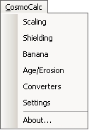
After installing the CosmoCalc add-in, a toolbar menu appears (Figure 1) that guides the user through the data reduction and closely follows the outline of this paper:
- Production rate scaling factors (Section 2)
- Lal (1991)
- Stone (2000)
- Dunai (2000)
- Desilets and Zreda (2003)
- Desilets et al. (2006)
- Shielding corrections (Section 3)
- Topographic shielding
- Self shielding
- Snow shielding
- Banana plots (Section 4)
- 26Al-10Be
- 21Ne-10Be
- Age/erosion rate calculations (Section 5)
- Single nuclide: exposure age and erosion rate calculations for 26Al, 10Be, 21Ne, 3He, 36Cl and 14C
- Two nuclides: simultaneous calculation of (burial or exposure) age and erosion rate.
- Converters (Section 6)
- Convert elevation to atmospheric pressure or -depth and back, under standard and Antarctic atmosphere.
- Convert geomagnetic latitude to -inclination or cutoff rigidity and back.
- Settings: customizing CosmoCalc (Section 7)
- Specify TCN production rate calibration sites
- Specify the relative importance of various production pathways
The following sections will provide more details about these calculations. Thus, the present paper serves as an abridged review of TCN calculations, with an emphasis on the numerical methods that are needed to solve the equations. More details about the physics of TCN production are given in the review article of Gosse and Philips (2001). CosmoCalc is not the first computational tool for TCN calculations. Useful alternatives are CHLOE, an Excel spreadsheet for cosmogenic 36Cl calculations (Phillips and Plummer, 1996) and the CRONUS-Earth web-calculator (Balco and Stone, 2007; http://hess.ess.washington.edu/math). CosmoCalc was developed independently from these other tools, except for its topographic shielding correction function, which was translated into VBA from the Matlab code of Balco and Stone (2007). The reader is strongly encouraged to try these other programs. CosmoCalc is optimized for 26Al, 10Be, 21Ne and 3He dating. Because geomagnetic field fluctuations and thermal neutron reactions are ignored, results for 36Cl and 14C may be inaccurate. CosmoCalc can be used as an exploratory tool for these nuclides, but for more accurate results, CHLOE or the spreadsheet of Lifton et al. (2005) are recommended.
2 Production rate scaling factors
In the simplest case (no shielding or burial), only three pieces of information are
needed to calculate an exposure age or erosion rate: TCN concentration, half-life and
production rate. Production rates are the “achilles heel” of the TCN method.
There exist only a few calibration sites where TCN production rates are
accurately known thanks to the availability of independent age constraints
(e.g., Nishiizumi et al., 1989; Niedermann et al., 1994; Kubik et al., 1998).
These production rates are only valid for the specific conditions (latitude,
elevation, age) of each particular calibration site. To apply the TCN method
to other field settings, the production rates must be scaled to a common
reference at sea level and high latitude (SLHL). Up to 20% uncertainty is
associated with this scaling, constituting the bulk of TCN age uncertainty.
Although several efforts have been made to directly measure TCN production
rate scaling with latitude and elevation using artificial H2O and SiO2 targets
(Nishiizumi et al., 1996; Brown et al., 2000; Graham et al., 2007), all currently used
scaling models are based on neutron monitor surveys. The oldest and still most
widely used scaling model is that of Lal (1991). This model is a simple set
of polynomial equations giving the (spallogenic + muogenic) production
rate relative to SLHL as a function of geographic latitude and elevation. In
CosmoCalc, Lal’s scaling factors can be calculated by simply selecting two columns
of latitude (in degrees) and elevation (in meters) data and clicking “OK”.
Lal’s scaling factors use elevation as a proxy for atmospheric depth, assuming a
standard atmosphere approximation. Stone (2000) noted that this approximation is
not valid in certain areas, such as Antarctica and Iceland. To avoid the systematic
errors caused by the standard atmosphere model, Stone (2000) recast the polynomial
equations of Lal (1991) in terms of air pressure instead of elevation. A second
improvement of the Stone (2000) model is the independent scaling of TCN
production by slow (negative) muons (Heisinger et al., 2002). In spite of this
added complexity, the CosmoCalc interface for Stone (2000) scaling factors is
identical to that for Lal (1991) scaling: the user simply needs to provide two
columns of data, one with latitude and one with air pressure (in mbar).
The scaling factors of Stone (2000) can be different for different nuclides,
because the importance of muons depends on the nuclide of interest. Because
most TCN production rate calibration sites are not located at SLHL, it is
crucially important to scale the production rates using the same method as the
unknown sample. This is exactly what CosmoCalc does when the user selects a
nuclide from the scroll-down menu of the scaling-form. Thus, the program
“forces” the user to be consistent. The program comes with a set of default
calibration sites, but these can be changed. Also the relative importance of the
production pathways (neutrons, slow and fast muons) can be changed (Section 7).
Behind the scaling models of both Lal (1991) and Stone (2000) lies an extensive
database of neutron monitor measurements, ordered according to geomagnetic
latitude. This ordering implies that Earth’s magnetic field can be accurately
approximated by a simple dipole. To avoid this approximation, Dunai (2000) ordered
the neutron monitor data according to geomagnetic inclination, which also represents
the non-dipole field. Just like Stone (2000), also Dunai (2000) incorporates
separate muon scaling and atmospheric effects. However, atmospheric depth
(g/cm2) is used instead of air pressure. Using CosmoCalc it is very easy to
convert air pressure to elevation or atmospheric depth and back (Section 6).
Ultimately, both geomagnetic latitude and inclination are merely proxies for a
more fundamental physical quantity: the geomagnetic cutoff rigidity (Rc), which is
the minimum momentum per unit charge (in GV), required for a primary cosmic ray
to reach the atmosphere. Ordering the neutron monitor data according to this
parameter results in yet another set of scaling factors. Unfortunately, at least three
different methods for calculating Rc exist in the literature. Dunai (2001) used a
database of horizontal magnetic field intensities and inclinations to estimate the
cutoff-rigidity of an equivalent axial dipole field, for which an approximate analytical
solution exists. Desilets and Zreda (2003) used a model based on trajectory tracing of
an axial dipole field, which is done by numerically testing the feasibility of vertically
incident anti-protons to travel from the top of the atmosphere back into space.
Finally, Lifton et al. (2005) fit a cosine function to a database of geomagnetic
latitudes versus trajectory traced cutoff rigidities for the 1955 magnetic
field. These authors consider the scatter around their fit to be a realistic
estimator of the natural variability of Rc at any given geomagnetic latitude.
In order to avoid confusion, CosmoCalc currently only implements one of these
three methods, namely that of Desilets and Zreda (2003). The scaling model of
Desilets and Zreda (2003) makes a distinction between slow and fast muons, each of
which scales differently. In an update of their model, Desilets et al. (2006) did a
neutron monitor survey at low latitudes, which were undersampled by previous
surveys. This resulted in a slightly different set of attenuation length polynomials for
spallogenic reactions. The method of Desilets et al. (2003, 2006) is probably the most
accurate of all the scaling models implemented in CosmoCalc. It is also the most
complex model, but this did not change the user interface. Using the scaling
models of Desilets et al. (2003, 2006) is just as easy as that of Lal (1991) in
CosmoCalc. Default values for the relative SLHL production rate contributions of
neutrons, slow and fast muons can be changed in the Settings menu (Section 7).
The scaling models of Dunai (2001), Desilets et al. (2003, 2006), Pigati and Lifton (2004), and Lifton et al. (2005) are a sensitive function of magnetic field intensity and solar activity, both of which are poorly constrained over geologic time. On the one hand, this temporal variability is the biggest downside to Rc-based models for long exposures (> 20 ka; Dunai, 2001). On the other hand, such models also offer the possibility to correct for secular variation of TCN production rates for short exposures. Instructions for doing so are given by Dunai (2001) and Desilets et al. (2003), provided a local record of paleomagnetic intensity is available. Compiling such a record is something for advanced users and falls beyond the scope of CosmoCalc. The scaling models of Pigati and Lifton (2004) and Lifton (2005) are accompanied by global datasets of magnetic field intensity, polar wander and solar activity and in principle, it would be possible to incorporate these datasets into CosmoCalc. However, because they are very large (4 and 7Mb, respectively) in comparison with CosmoCalc (~ 500kb), the cost of including these scaling models was considered too high. Therefore, researchers working with 14C, where secular variation of the magnetic field is really crucial, should use CosmoCalc only as an exploratory tool, and use the spreadsheets of Pigati and Lifton (2004) and Lifton et al. (2005) for final calculations.
3 Shielding corrections
The scaling factors discussed in the previous section allow the calculation of TCN production rates at any location on the Earth’s surface, assuming that the sample is a slab of zero thickness taken from a horizontal planar surface. If these assumption are not fulfilled, the SLHL production rates must be multiplied by a second set of correction factors, quantifying the extent to which the cosmic rays were blocked. CosmoCalc implements three such correction factors: topographic shielding, self shielding and snow cover.
3.1 Topographic shielding
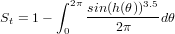
Two kinds of topographic shielding corrections can be distinguished for (a) samples taken from a tilted rather than horizontal surface, and (b) samples that are located in the vicinity of topographic irregularities. CosmoCalc follows the approach of Balco and Stone (2007) (their Matlab function skyline.m) and treats these two effects together using the following equation:
 | (1) |
With h(θ) the “horizon” in the azimuthal direction θ, i.e. either the elevation (in radians) of the topography or the sloping sample surface, whichever is greatest. Sometimes, an exponent of 2.3 is used instead of 3.5 in Equation 1 (Staudacher and Allègre, 1993). CosmoCalc treats this exponent as a variable, which can be changed in the Settings form (Section 7). In practice, the integral of Equation 1 is solved by linear interpolation between a finite number of azimuth/elevation measurements. The input needed by CosmoCalc is two mandatory columns of strike and dip (in degrees, where the strike is 90 degrees less than the direction of the dip), followed by an optional series of topographic azimuth/elevation measurements (in degrees). There is no restriction on the total number of measurements, provided they come in multiples of two.
3.2 Self-shielding
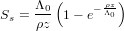
Cosmic rays are rapidly attenuated as they travel through matter, causing TCN production rates to vary greatly with depth below the rock/air contact. They must be integrated over the actual sample thickness and scaled to the surface production rates before an exposure age can be calculated. Different reaction mechanisms are associated with different attenuation lengths. Gosse and Philips (2001) consider four kinds of thickness corrections, for spallogenic, thermal and epithermal neutrons, and muons. Because self-shielding corrections are generally small, CosmoCalc considers only the spallogenic neutron reactions:
 | (2) |
with Λ0 the spallogenic neutron attenuation length (default value 160 g/cm2), ρ the rock density (default value 2.65 g/cm3) and z the sample thickness (in cm). Neglecting the remaining pathways makes little difference, with the possible exception of 36Cl, because the latter can be strongly affected by thermal neutron fluxes, which are currently ignored by CosmoCalc.
3.3 Snow cover
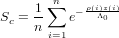
Perhaps the most popular and powerful application of TCN techniques is the dating of glacial moraines (e.g., Gosse et al., 1995; Schäfer et al., 1999). These features are generally located at high latitudes or elevations, where snow cover poses a potential problem. The snow correction is similar to the self-shielding correction with the important difference that the former is highly variable with time. Given n (e.g., 12 for monthly or 4 for seasonal) measurements of average snow thickness z and density ρ, CosmoCalc computes the snow correction factor Sc as follows:
 | (3) |
4 Banana plots
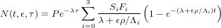
Before calculating an exposure age or erosion rate, it is a good idea to check if the TCN measurements are consistent with a simple or complex exposure history. This can be done with two nuclides (including at least one radionuclide) using a “banana plot” (Lal, 1991). CosmoCalc accomodates two types of banana plot: 26Al-10Be and 21Ne-10Be. Depending on whether or not a sample plots above, below or inside the so-called “steady-state erosion island” (Lal, 1991), one can decide whether or not to pursue the calculation of an exposure age, erosion rate or burial age. For the construction of the banana plots and the age/erosion calculations of Section 5, CosmoCalc implements a modified version of the ingrowth equation of Granger and Muzikar (2001):
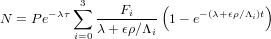 | (4) |
With N the nuclide concentration (atoms/g), P the total surface production rate
(in atoms/g/yr) at SLHL, τ the burial age, ϵ the erosion rate, t the exposure age and
λ the radioactive half-life of the nuclide. Equation 4 models TCN production by
neutrons, slow and fast muons by a series of exponential approximations. The first
term of the summation models TCN production by spallogenic neutron reactions, the
second and third terms model slow muons and the last term approximates TCN
production by fast muons. Thus, F0,...,F3 are dimensionless numbers between zero
and one, and Λ0,...,Λ3 are attenuation lengths (g/cm2). The approach of Granger et
al. (2000, 2001) was chosen because of its flexibility. For instance, neglecting muon
production can be easily implemented by setting F1,F2 and F3 equal to zero in
Equation 4. CosmoCalc uses Granger et al.’s (2000, 2001) recommended
values of F0,...,F3 for 10Be and 26Al, but also offers an alternative choice
of pre-set values approximating either the alternative parameterization of
Schaller et al. (2001), neglecting the contribution of muons, or only using three
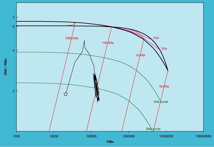
exponentials (for more details, see Section 7). Banana plots with non-zero
muon contributions feature a characteristic cross-over of the steady-state and
zero erosion lines which is absent when muons are neglected (Figure 2).
CosmoCalc’s banana plots are normalized to SLHL, meaning that the TCN concentrations of each sample are divided by the cumulative effect of all their correction factors, represented by the “effective scaling factor” Se:
 | (5) |
with
 | (6) |
where Sp is one of the production rate scaling factors of Section 2 and St, Ss and
Sc are defined in Section 3. If muon production is neglected, then Se = St × Sp × Ss
× Sc. However, in the presence of muons, the effective scaling factor Se may deviate
from this value because the relative importance of the different production
mechanisms changes as a function of age, erosion rate, elevation, latitude, sample
thickness and snow cover. The exact form of the function f(S) will be defined in
Section 5.2.4. Note that the topographic shielding correction St does not
“fractionate” (i.e., change the fractions F0,...,F3 of) the different production
mechanisms and is placed outside the scaling function f(S). This means that, strictly
speaking, the TCN concentrations should be multiplied by St prior to generating a
banana plot. The input required by CosmoCalc’s “Banana” function are (1)
the composite scaling factor S for the first nuclide (26Al or 21Ne), (2) the
concentration and 1σ measurement uncertainty of the first nuclide (26Al or
21Ne), both multiplied by St, (3) S for the second nuclide (10Be) and (4)
the concentration and 1σ measurement uncertainty of the second nuclide
(10Be), also multiplied by St. Because topographic shielding corrections are
generally small, the systematic error caused by lumping St together with
the other correction factors is very small. Therefore, if St > ~ 0.95, say, it
is safe to approximate Equation 5 by Se = f(St × Sp × Ss × Sc). In this
case, the nuclide concentrations do not need to be pre-multiplied by St.
a.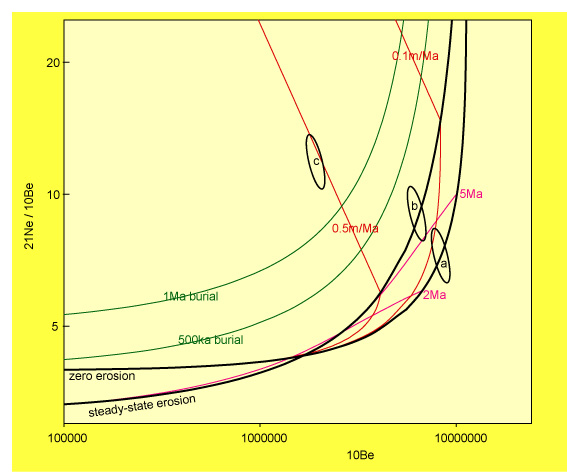 b.
b.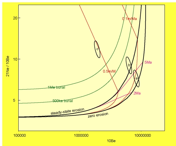
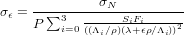
The graphical output of CosmoCalc can easily be copied and pasted for editing in vector graphics software such as Adobe Illustrator or CorelDraw. The y-axis of the 26Al-10Be plot is logarithmic by default whereas the y-axis of the 21Ne-10Be plot is linear. These defaults can be changed in the “Banana Options” userform. Note that MS-Excel (versions 2000 and 2003) only allows logarithmic tickmarks to have values in multiples of ten. To get around this limitation, CosmoCalc uses a “pseudo y-axis”, which cannot be edited by the usual right mousebutton-click. Hopefully, this limitation will not be necessary in later versions of Excel. CosmoCalc only propagates the analytical uncertainty of the measured TCN concentrations. No uncertainty is assigned to the production rate scaling factors, radioactive half-lives or other potentially ill-constrained quantities. On the banana plots, the user is offered the choice between error bars or -ellipses with the latter being the default. Banana plots are graphs of the type N1/N2 vs. N2 which are always associated with some degree of “spurious correlation” (Chayes, 1949). This causes the error ellipses to be rotated according to the following correlation coefficient:
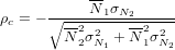 | (7) |
If N1 stands for 26Al or 21Ne and N2 for 10Be, then N1 and N2 are the measured concentrations of these respective nuclides while σN1 and σN2 are the corresponding measurement uncertainties.
5 Age/erosion rate calculations
Equation 4 has three unknowns: t (exposure age), ϵ (erosion rate) and τ (burial age). If only one nuclide was measured, we must assume values for two of these quantities in order to solve for the third. If two nuclides were analysed (of which at least one is radioactive), only one assumption is needed. CosmoCalc is capable of both approaches. In this section, we will first discuss how to solve for ϵ (assuming infinite exposure age and zero burial) and t (assuming zero erosion and burial) using a single nuclide (Section 5.1). Then, numerical methods will be presented to simultaneously solve for t and ϵ (assuming zero burial), t and τ (assuming zero erosion) or ϵ and τ (assuming infinite exposure age), using two nuclides (Section 5.2). Note that in the case of two nuclides (26Al or 21Ne combined with 10Be), the assumption of zero burial can be verified on the banana plot.
5.1 Calculations using a single nuclide
CosmoCalc requires three pieces of information to calculate an exposure age or erosion rate: the TCN concentration (corrected for topography), its analytical uncertainty and a composite correction factor for production rate scaling with latitude/elevation and shielding (Equation 6). We somehow need to incorporate this scaling factor into the ingrowth equation (Equation 4). This poses a problem because the scaling factor is a single number whereas Equation 4 explicitly makes the distinction between neutrons, slow and fast muons. Granger and Smith (2000) avoid this problem by separately scaling the different production mechanisms:
 | (8) |
Instead of one scaling factor, Equation 8 has four, one for neutrons (S0), two for slow muons (S1 and S2) and one for fast muons (S3). Granger et al. (2001) separately calculate each of these four scaling factors. Thus, the original method of Granger and Smith (2000) is incompatible with the common practice of lumping all production mechanisms into a single latitude/elevation scaling factor (Section 2). To ensure optimal flexibility and user-friendliness, CosmoCalc uses a slightly different approach. S0,...,S3 are calculated from the composite correction factor S, by approximating the total scaling by a single attenuation factor caused by a virtual layer of matter of thickness x (in g/cm2):
 | (9) |
so that
 | (10) |
with Fi and Λi as in Equation 4 and S as defined in Equation 6. CosmoCalc
solves Equation 10 iteratively using Newton’s method.
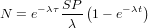
As said before, some assumptions are needed to solve Equation 8. An exposure age (t) can be calculated under the assumption of zero erosion and burial (ϵ = 0, τ = 0). For a radionuclide with decay constant λ, this yields:
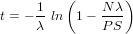 | (11) |
whereas for stable nuclides (3He and 21Ne):
 | (12) |
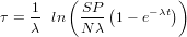
Alternatively, the erosion rate (ϵ) can be calculated under the assumption of steady state and zero burial (t = ∞, τ=0):
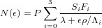 | (13) |
CosmoCalc solves this equation iteratively using Newton’s method. Statistical uncertainties are estimated by standard error propagation:
 | (14) |
 | (15) |
These error estimates do not include any uncertainties in production rates and scaling factors, which are difficult to quantify, but can be evaluated by using a range of input parameters.
5.2 Calculations with two nuclides
Equation 8 has three unknowns (t, ϵ and τ). If two nuclides have been measured (with concentrations N1 and N2, say), only one value must be assumed in order to solve for the remaining two. By assuming zero erosion (ϵ = 0), CosmoCalc simultaneously calculates the exposure age and burial age (Section 5.2.1); by assuming steady-state erosion (t = ∞), the erosion rate and burial age are calculated; and by assuming zero-burial (τ = 0), the erosion rate and exposure age can be computed (Section 5.2.2).
5.2.1 Burial dating
If a rock surface gets buried by sediments or covered by ice, it is shielded from cosmic rays and the concentration of cosmogenic radionuclides decays with time. Such samples plot outside the steady-state erosion island of the banana plot, in the so-called field of “complex exposure history”, a feature which is considered undesirable by most studies. Other studies, however, intentionally target complex exposure histories, using radionuclides to date pre-exposure and burial (e.g., Bierman et al., 1999; Fabel et al., 2002; Partridge et al., 2003). CosmoCalc calculates burial ages, either by assuming negligible erosion or steady state erosion (ϵ = 0 or t = ∞, respectively). It does not handle post-depositional nuclide production.
Burial - Exposure dating
If ϵ = 0, Equation 8 reduces to:
 | (16) |
The easiest case of two-nuclide dating is that of simultaneously calculating exposure age (t) and burial age (τ) with one radionuclide and one stable nuclide. Because the stable nuclide is not affected by burial, it can be used to calculate the pre-exposure age, using Equation 12. This age can then be used to calculate the burial age:
 | (17) |
In the case of two radionuclides, CosmoCalc finds t by iteratively solving the following equation using Newton’s method:
 | (18) |
With λ1 > λ2. The solution is then plugged into Equation 17, using nuclide 1.
Burial - Erosion dating
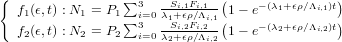
Setting t = ∞ in Equation 8 yields the following system of non-linear equations
for TCN concentrations N1 and N2:
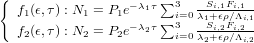 | (19) |
These equations are easy to solve since the variables τ and ϵ are separated. If nuclide 1 has the shortest half-life (largest decay constant λ), the burial age is written as a function of the erosion rate ϵ:
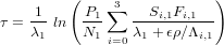 | (20) |
The erosion rate is given implicitly by:
 | (21) |
CosmoCalc solves Equation 21 for ϵ using Newton’s method and then plugs this value into Equation 20. If λ2 < λ1, then N2 is used instead of N1 in Equation 20.
5.2.2 Age-erosion rate calculations
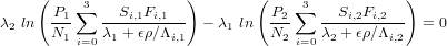
Assuming zero burial (τ = 0) yields the following system of equations f1 and f2:
 | (22) |
It is impossible to solve these equations for exposure age (t) and erosion rate (ϵ) separately. Instead, CosmoCalc implements the two-dimensional version of the Newton-Raphson algorithm:
![[ ] [ ] ⌊ ( ) ( ) ⌋ -1[ ]
ϵk+1 ϵk ⌈a = (∂f∂1ϵ)k b = ( ∂∂f1t)k⌉ f1(ϵk,tk)
tk+1 = tk - c = ∂f2 d = ∂f2- f2(ϵk,tk)
∂ϵ k ∂t k](CosmoPaper24x.png) | (23) |
With J(ϵ,t) = ![[ ]
a b
c d](CosmoPaper25x.png) the Jacobian matrix, which is also used for error
propagation.
the Jacobian matrix, which is also used for error
propagation.
5.2.3 Error propagation
Error propagation is less straightforward in the two-dimensional case than in the single nuclide case (Section 5.1). The bijection from (N1,N2)-space to (ϵ,t)-space is not orthogonal, particularly in the case of age-erosion dating (Section 5.2.2). For this reason, it is only possible to analytically compute upper bounds for σ(ϵ), σ(τ) and σ(t):
![[ ] [ ]
σ(x) ∥∥ -1∥∥ σ(N1 )
σ(y) ≤ J(x,y) σ(N2 )](CosmoPaper26x.png) | (24) |
with x and y placeholders for ϵ and t or τ, respectively, and ∥⋅∥ the absolute
values of the matrix ![[⋅]](CosmoPaper27x.png) . In the case of age-erosion dating, the confidence intervals for
t and ϵ are very wide, often too wide to be useful. Therefore, it can be more
productive to solve each quantity separately instead of simultaneously. Thus, using
equations 11 and 13, it is possible to estimate minimum exposure ages and
maximum erosion rates (e.g., Nishiizumi et al., 1991). However, for burial
dating there is no choice and we must simultaneously solve for τ and ϵ or t.
. In the case of age-erosion dating, the confidence intervals for
t and ϵ are very wide, often too wide to be useful. Therefore, it can be more
productive to solve each quantity separately instead of simultaneously. Thus, using
equations 11 and 13, it is possible to estimate minimum exposure ages and
maximum erosion rates (e.g., Nishiizumi et al., 1991). However, for burial
dating there is no choice and we must simultaneously solve for τ and ϵ or t.
In addition to Newton’s method, CosmoCalc offers a second way of solving equations 19 and 22 by means of Monte Carlo simulation, implementing the Metropolis-Hastings algorithm (Metropolis et al., 1953; Tarantola, 2004). The Metropolis-Hastings algorithm is a so-called Bayesian MCMC (Markov Chain Monte Carlo) method. It not only finds the best solution to the system of non-linear equations, but actually explores the entire solution space. If the “Metropolis” option of the Age-Erosion function is selected, CosmoCalc generates 1000 “acceptable” solutions to Equation 19 or 22, where “acceptable” is defined by the bivariate normal likelihood of the forward-modeled TCN concentrations (Figure 3). The last 900 of these solutions are then ranked according to their likelihood. For a 95% confidence interval, those solutions with the lowest 5% likelihoods of the 900 results are discarded, leaving 855 values for ϵ, t or τ. The minimum and maximum values of these 855 numbers are the lower and upper bounds, respectively, of the simultaneous 95% confidence intervals. In contrast with the symmetric confidence intervals given by equation 24, the MCMC confidence limits are always greater than or equal to zero. However, as said before, the 95% confidence intervals can be very wide especially in the case of age-erosion dating.
5.2.4 An a posteriori modification of the banana plots
Section 4 discussed the construction of 26Al-10Be and 21Ne-10Be banana plots. To plot samples from different field locations (with different latitude, elevation and shielding conditions) together on the same banana plot, it is necessary to scale the TCN concentrations to SLHL. In other words, each TCN concentration must be divided by an appropriate scaling factor, the so-called “effective scaling factor” Se (Equation 5):
 | (25) |
With Nmeas the measured TCN concentration, and NSLHL the equivalent TCN concentration which would be measured had the sample been collected from SLHL. In the case of zero erosion, NSLHL = Nmeas / (Sp × St × Ss × Sc). This is no longer true when ϵ > 0, because the relative contributions of neutron spallation, slow and fast muons change below the surface. This is the “fractionation” effect that was discussed in Section 4 and quantified by Equation 10. For example, consider the case of two high latitude, high elevation samples, one with negligible erosion (ϵ=0) and one with non-zero erosion (ϵ>0). Because the relative importance of neutron spallation increases with decreasing erosion rate, and neutrons are more important (relative to muons) at higher elevations, Se will be greater for the zero-erosion than for the non-zero erosion case. CosmoCalc first solves Equation 19 or 22 for ϵ and τ or t, whichever fits the measured TCN concentrations best. Plugging these solutions into Equation 4 yields the equivalent TCN concentration at SLHL. Se is then given by Equation 25.
6 Converters
Section 2 discussed four different models to scale TCN production rates from SLHL
to any other location on Earth. All these models have in common that they require
two columns of data in CosmoCalc: “latitude” and “elevation”. They differ in
how they quantify these two pieces of information. The scaling factors of
Lal (1991) are the only ones that use the actual geographical latitude (in
degrees) and elevation (in meters). Stone (2000) also uses the geographical
latitude for estimating the latitude effect, but uses atmospheric pressure (in
mbar) for modeling the elevation effect. Dunai (2000) uses the geomagnetic
inclination (in degrees) instead of latitude, and atmospheric depth (in g/cm2)
instead of elevation. Finally, Desilets et al. (2003, 2006) use cut-off rigidity (in
GV) for the latitude effect and atmospheric depth for the elevation effect.
All these different measures of “latitude” and “elevation” are related to each other and can be converted into each other. To facilitate the comparison of the different methods and, for example, reinterpret published literature data, CosmoCalc provides a series of easy-to-use conversion tools.
6.1 Converting different measures of “elevation”
To convert elevation (z, in m) to atmospheric pressure (p, in mbar) (Iribane and Godson, 1992):
 | (26) |
With p0 the pressure at sea level, β0 the adiabatic lapse rate, T0 the temperature at sea level, g0 the gravitational constant and Rd the universal gas constant. In the standard atmospheric model, β0 = 6.5 K/km, g0 = 9.80665 m/s2, p0 = 1013.25 mbar and T0 = 288.15 K. However, these values are not valid for Antarctica, where p0 ≈ 989.1 mbar and T0 ≈ 250 K. The modified Equation 26 can be rewritten as (Stone, 2000):
 | (27) |
Atmospheric pressure is converted to atmospheric depth (g/cm2) by:
 | (28) |
The reverse conversions are trivial inversions of these equations.
6.2 Converting different measures of “latitude”
Converting latitude (L, in degrees) to geomagnetic inclination (I, in degrees) and back:
 | (29) |
Converting latitude to geomagnetic cut-off rigidity (in GV) for a geomagnetic field strength M, compared to the 1945 reference value (M0 = 8.085×10² A m2):
 | (30) |
The default value for M/M0 = 1, but can be changed by clicking the “Option” button of the CosmoCalc conversion form. e1,...,e6 and f1,...,f6 are defined in Table 8 of Desilets and Zreda (2003). The reverse operation of Equation 30 does not have an analytical solution and is solved iteratively with Newton’s method.
7 Customizing CosmoCalc
The interface of CosmoCalc is very simple because default values are set for most of the parameters that occur in the various equations discussed in this paper (Table 1). This greatly reduces the chance that novice users make mistakes when reducing their TCN data. For more advanced users, the program allows nearly all the parameters to be changed.
7.1 Specifying the production rate calibration sites
As mentioned in Section 2, it is very important to use a consistent set of scaling factors for the unknown sample and the production rate calibration site. Failing to do so can cause significant systematic errors. To avoid this, CosmoCalc defines the SLHL production rates implicitly, by specifying a set of calibration sites and their measured TCN concentrations. Using the “Calibration sites” form of the “Settings” menu, these concentrations are scaled to SLHL and an average production rate is calculated using one of the five scaling models of Section 2. CosmoCalc comes with a default set of published production rate calibrations, some of which (10Be and 26Al) were borrowed from Balco and Stone (2007; http://hess.ess.washington.edu/math). The published data come from a variety of latitudes and elevations, yielding a presumably reliable estimate of the globally averaged production rates. This, however, is not always the best approach. For example, if a TCN study is carried out in the vicinity of one particular calibration site, then it makes more sense to use only this site to estimate the local production rate. Therefore, CosmoCalc offers the user the flexibility to delete or add calibration sites at will.
7.2 Changing the relative contributions of different production pathways
Being based on the equation of Granger and Smith (2000), the TCN production
equation consists of four exponentials: one for neutrons, two for slow neutrons, and
one for fast neutrons (see Equation 8 and Section 5). These exponentials are governed
by two sets of parameters: the fractions Fi and the attenuation lengths Λi (for
i=0,...,3). Default values for Λi, Fi(10Be) and Fi(26Al) were taken from Granger and
Smith (2000) (Table 1), but these values can be changed in the “Settings” form.
| parameter | symbol | default value | units |
| rock density | ρ | 2.65 | g/cm3 |
| decay constant (10Be) | λ(10Be) | 4.560E-07 | yr-1 |
| decay constant (26Al) | λ(26Al) | 9.800E-07 | yr-1 |
| decay constant (36Cl) | λ(36Cl) | 2.300E-06 | yr-1 |
| decay constant (14C) | λ(14C) | 1.213E-04 | yr-1 |
| attenuation length (neutrons) | Λ0 | 160 | g/cm2 |
| attenuation length (slow muons) | Λ1 | 738 | g/cm2 |
| attenuation length (slow muons) | Λ2 | 2688 | g/cm2 |
| attenuation length (fast muons) | Λ3 | 4360 | g/cm2 |
| relative production by neutrons (10Be) | F0(10Be) | 0.9724 | – |
| relative production by neutrons (26Al) | F0(26Al) | 0.9655 | – |
| relative production by neutrons (14C) | F0(14C) | 0.83 | – |
| relative production by neutrons (36Cl) | F0(36Cl) | 0.903 | – |
| relative production by neutrons (3He) | F0(3He) | 1 | – |
| relative production by neutrons (21Ne) | F0(21Ne) | 1 | – |
| relative production by slow muons (10Be) | F1(10Be) | 0.0186 | – |
| relative production by slow muons (26Al) | F1(26Al) | 0.0233 | – |
| relative production by slow muons (14C) | F1(14C) | 0.0691 | – |
| relative production by slow muons (36Cl) | F1(36Cl) | 0.0447 | – |
| relative production by slow muons (3He) | F1(3He) | 0 | – |
| relative production by slow muons (21Ne) | F1(21Ne) | 0 | – |
| relative production by slow muons (10Be) | F2(10Be) | 0.004 | – |
| relative production by slow muons (26Al) | F2(26Al) | 0.005 | – |
| relative production by slow muons (14C) | F2(14C) | 0.0809 | – |
| relative production by slow muons (36Cl) | F2(36Cl) | 0.0523 | – |
| relative production by slow muons (3He) | F2(3He) | 0 | – |
| relative production by slow muons (21Ne) | F2(21Ne) | 0 | – |
| relative production by fast muons (10Be) | F3(10Be) | 0.005 | – |
| relative production by fast muons (26Al) | F3(26Al) | 0.0062 | – |
| relative production by fast muons (14C) | F3(14C) | 0.02 | – |
| relative production by fast muons (36Cl) | F3(36Cl) | 0 | – |
| relative production by fast muons (3He) | F3(3He) | 0 | – |
| relative production by fast muons (21Ne) | F3(21Ne) | 0 | – |
| sea level temperature | T0 | 288.15 | K |
| adiabatic lapse rate | β0 | 6.5 | K/km |
| air pressure at sea level | P0 | 1013.25 | mbar |
| geomagnetic field intensity relative to 1945 | M/M0 | 1 | – |
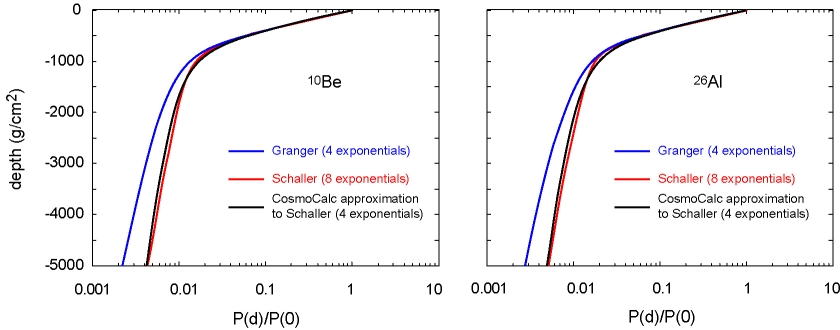
In addition to Equation 8, several alternative, but similar looking TCN ingrowth equations exist in the literature. Schaller et al. (2001, 2002) use not four but eight exponentials (two for neutrons, and three for each slow and fast muons), whereas others use three (one for each production mechanism) (e.g., Braucher et al., 2003; Miller et al., 2006) or only one exponential (neglecting muon production). CosmoCalc provides a separate set of default parameters for each of these alternatives. For example, the ingrowth equation of Schaller et al. (2002) was recast in the parameterization of Granger and Smith (2000) by a least squares fit of a virtual depth profile (Figure 4).
8 How to report data reduced with CosmoCalc
CosmoCalc was designed to be a user-friendly program for both novice and advanced
users of TCN methods. Nearly every function comes with a set of options which allow
the user to change the default values of various parameters (Section 7). Although
CosmoCalc’s flexibility should be considered a positive feature, a danger exists that
his may lead to confusion. Therefore, it is important that the data-reduction
method is well documented when reporting results. Here is an example:
“Ages were calculated with CosmoCalc 1.0 (Vermeesch, 2007), using Dunai
(2000) scaling factors and default values for all parameters with the following
exceptions: ρ = 3.5 g/cm3 and λ(10Be) = 5.17×10⁻⁷yr-1.”
Clearly indicating the version number is important because CosmoCalc
will be updated in the future to keep track of new developments in TCN
geochronology. Older versions will always be available from the CosmoCalc website
(http://cosmocalc.googlepages.com). Users with useful suggestions for improvements
should feel free contact the author by emailing to cosmocalc@gmail.com.
Acknowledgments. The author is financially supported by a Marie Curie Fellowship of the European Union (CRONUS-EU network, RTN project reference 511927). Many thanks to Dr. Naki Akçar for testing beta-versions of CosmoCalc and making useful suggestions which simplified the user interface and made the program more user-friendly, and to two anonymous reviewers for constructive comments.
References
- Balco, G., and J.O.H. Stone, A simple, internally consistent, and easily accessible means of calculating surface exposure ages or erosion rates from 10Be and 26Al measurements, Quaternary Geochronology, (in preparation).
- Bierman, P.R., K.A. Marsella, C. Patterson, P.T. Davis, and M. Caffee, Mid-Pleistocene cosmogenic minimum-age limits for pre-Wisconsian glacial surfaces in southwestern Minnesota and southern Baffin island: a multiple nuclide approach, Geomorphology, 27 (1-2), 25-39, 1999.
- Braucher, R., E.T. Brown, D.L. Bourles, and F. Colin, In situ produced 10Be measurements at great depths: implications for production rates by fast muons, Earth and Planetary Science Letters, 211, 251-258, 2003.
- Brown, E.T., T.W. Trull, P. Jean-Baptiste, G. Raisbeck, D. Bourles, F. Yiou, and B. Marty, Determination of cosmogenic production rates of 10Be, 3He and 3H in water, Nuclear Instruments and Methods in Physics Research B, 172, 802-805, 2000.
- Chayes, F., On ratio correlation in petrography, Journal of Geology, 57 (3), 239-254, 1949.
- Desilets, D., and M. Zreda, Spatial and temporal distribution of secondary cosmic-ray nucleon intensities and applications to in situ cosmogenic dating, Earth and Planetary Science Letters, 206, 21-42, 2003.
- Desilets, D., M. Zreda, and T. Prabu, Extended scaling factors for in situ cosmogenic nuclides: New measurements at low latitude, Earth and Planetary Science Letters, 246, 265-276, 2006.
- Dunai, T.J., Scaling factors for production rates of in situ produced cosmogenic nuclides: a critical reevaluation, Earth and Planetary Science Letters, 176, 157-169, 2000.
- Dunai, T.J., Influence of secular variation of the geomagnetic field on production rates of in situ produced cosmogenic nuclides, Earth and Planetary Science Letters, 193, 197-212, 2001.
- Dunai, T.J., and Wijbrans J.R., Long-term 3He production rates (152 ka - 1.35 Ma) from 40Ar/39Ar dated basalt flows at 29o latitude, Earth and Planetary Science Letters, 176, 147-156, 2000.
- Fabel, D., A.P. Stroeven, J. Harbor, J. Kleman, D. Elmore, and D. Fink, Landscape preservation under Fennoscandian ice sheets determined from in situ produced 10Be and 26Al, Earth and Planetary Science Letters, 201, 397-406, 2002.
- Graham, I.J., Barry, B.J., Ditchburn, R.G., Whitehead, N.E., Zondervan, A., Direct measurement of cosmogenic production of 7Be and 10Be in water targets in the southern hemisphere, Earth and Planetary Science Letters (in preparation)
- Granger, D.E., and A.L. Smith, Dating buried sediments using radioactive decay and muogenic production of 26Al and 10Be, Nuclear Instruments and Methods in Physics Research B, 172, 822-826, 2000.
- Granger, D.E., C.S. Riebe, J.W. Kirchner, and R.C. Finkel, Modulation of erosion on steep granitic slopes by boulder armoring, as revealed by cosmogenic 26Al and 10Be, Earth and Planetary Science Letters, 186, 269-281, 2001.
- Granger, D.E., and P.F. Muzikar, Dating sediment burial with in situ-produced cosmogenic nuclides: theory, techniques, and limitations, Earth and Planetary Science Letters, 188, 269-281, 2001.
- Gosse, J.C., E.B. Evenson, J. Klein, B. Lawn, and R. Middleton, Precise cosmogenic 10Be measurements in western North America: Support for a global Younger Dryas cooling event, Geology, 23, 877-880, 1995.
- Gosse, J.C., and F.M. Phillips, Terrestrial in situ cosmogenic nuclides: theory and application, Quaternary Science Reviews, 20, 1475-1560, 2001.
- Heisinger, B., D. Lal, A.J. Jull, S. Ivy-Ochs, S. Neumaier, K. Knie, V. Lazarev, and E. Nolte, Production of selected cosmogenic radionuclides by muons: 1. Fast Muons, Earth and Planetary Science Letters, 200, 345-355, 2002.
- Heisinger, B., D. Lal, A.J. Jull, P.W. Kubik, S. Ivy-Ochs, K. Knie, and E. Nolte, Production of selected cosmogenic radionuclides by muons: 2. Capture of negative muons, Earth and Planetary Science Letters, 200, 357-369, 2002.
- Iribane, J.V., and W.L. Godson, Atmospheric Thermodynamics, 259 pp., D. Reidel, Dordrecht, 1992.
- Kubik, P.W., S. Ivy-Ochs, J. Masarik, M. Frank, and C. Schlüchter, 10Be and 26Al production rates deduced from an instantaneous event within the dendro-calibration curve, the landslide of Köfels, &OUML;tz Valley Austria, Earth and Planetary Science Letters, 161, 231-241, 1998.
- Kurz, M.D., Cosmogenic helium in terrestrial igneous rock, Nature, 320, 435-439, 1986.
- Lifton, N.A., J.W. Bieber, J.M. Clem, M.L. Dulding, P. Evenson, J.E. Humble, and R. Pyle, Addressing solar modulation and long-term uncertainties in scaling secondary cosmic rays for in situ cosmogenic nuclide applications, Earth and Planetary Science Letters, 239, 140-161, 2005.
- Lal, D., Cosmic ray labeling of erosion surfaces: in situ nuclide production rates and erosion models, Earth and Planetary Science Letters, 104, 424-439, 1991.
- Metropolis, N., A.W. Rosenbluth, M.N. Rosenbluth, A.H. Teller, and E. Teller, Equations of state calculations by fast computing machines, Journal of Chemical Physics, 21, 1087-192, 1953.
- Miller, G.H., J.P. Briner, N.A. Lifton, and R.C. Finkel, Limited ice-sheet erosion and complex exposure histories derived from in situ cosmogenic 10Be, 26Al, and 14C on Baffin Island, Arctic Canada, Quaternary Geochronology, 1, 74-85, 2006.
- Niedermann, S., T. Graf, J.S. Kim, C.P. Kohl, K. Marti, and K. Nishiizumi, Cosmic-ray produced 21Ne in terrestrial quartz: the neon inventory of Sierra Nevada quartz separates, Earth and Planetary Science Letters, 125, 341-355, 1994.
- Nishiizumi, K., D. Lal, J. Klein, R. Middleton, and J.R. Arnold, Production of 10Be and 26Al by cosmic rays in terrestrial quartz in situ and implications for erosion rates, Nature, 319, 134-135, 1986.
- Nishiizumi, K., E. L. Winterer, et al. Cosmic ray production rates of 10Be and 26Al in quartz from glacially polished rocks. Journal of Geophysical Research, 94, 17907-17915, 1989.
- Nishiizumi, K., C.P. Kohl, J.R. Arnold, J. Klein, D. Fink, and R. Middleton, Cosmic ray produced 10Be and 26Al in Antarctic rocks: exposure and erosion history, Earth and Planetary Science Letters, 104, 440-454, 1991.
- Nishiizumi, K., R.C. Finkel, J. Klein, and C.P. Kohl, Cosmogenic production of 7Be and 10Be in water targets, Journal of Geophysical Research., 101, 22225-22232, 1996.
- Partridge, T.C., D.E. Granger, M.W. Caffee, and R.J. Clarke, Lower Pliocene hominid remains from Sterkfontein, Science, 300, 607-612, 2003.
- Phillips, F.M., B.D. Leavy, N.O. Jannik, D. Elmore, and P.W. Kubik, The accumulation of cosmogenic Chlorine in rocks: a method for surface exposure dating, Science, 231, 41-43, 1986.
- Phillips, F.M., and M.A. Plummer, CHLOE: A program for interpreting in situ cosmogenic nuclide data for surface exposure dating and erosion studies, Radiocarbon, 38, 98, 1996.
- Pigati, J.S., and N.A. Lifton, Geomagnetic effects on time-integrated cosmogenic nuclide production with emphasis on in situ 14C and 10Be, Earth and Planetary Science Letters, 226, 193-205, 2004.
- Schäfer, J.M., S. Ivy-Ochs, R. Wieler, I. Leya, H. Baur, G.H. Denton, and C. Schlüchter, Cosmogenic noble gas studies in the oldest landscape on earth: surface exposure ages of the Dry Valleys, Antarctica, Earth and Planetary Science Letters, 167, 215-226, 1999.
- Schaller, M., F. von Blanckenburg, N. Hovius, and P.W. Kubik, Large-scale erosion rates from in situ-produced cosmogenic nuclides in European river sediments, Earth and Planetary Science Letters, 188, 441-458, 2001.
- Schaller, M., F. von Blanckenburg, A. Veldkamp, L.A. Tebbens, N. Hovius, and P.W. Kubik, A 30000yr record of erosion rates from cosmogenic 10Be in Middle Europe river terraces, Earth and Planetary Science Letters, 204, 307-320, 2002.
- Staudacher, T., and C.J. Allègre, Ages of the second caldera of Piton de la Fournaise volcano (Réunion) determined by cosmic ray produced 3He and 21Ne, Earth and Planetary Science Letters, 119, 395-404, 1993.
- Stone, J.O., G.L. Allan, L.K. Fifield, and R.G. Cresswell, Cosmogenic chlorine-36 from calcium spallation, Geochimica et Cosmochimica Acta, 60, 555-561, 1996.
- Stone, J., Air pressure and cosmogenic isotope production, Journal of Geophysical Research, 105, 23753-23759, 2000.
- Tarantola, A., Inverse problem theory, 342 pp., Society for Industrial and Applied Mathematics, 2004.