Have you ever wondered how plastic bags are made?
Dr. Helen Wilson
from UCL's Mathematics department is working with colleagues around
the country on the Microscale Polymer Processing project to make
the process more reliable.
Plastics are made from very long molecules called polymers, thousands
or millions of times bigger than a simple molecule like carbon
dioxide, water or methane. They are usually processed in a liquid
state, at high temperatures and pressures.

These long molecules naturally tend to coil up in their liquid state,
because of Brownian motion. But when the liquid is being processed -
say, extruded into a thin film to make bags - these coils can get
stretched out. Their natural tendency to retract back to a coiled
shape gives the liquid an elasticity - like the stringiness of
cheese on a pizza.
The equations that describe the flow of a melted plastic are
complicated - so complicated, in fact, that there is no perfect set
of equations for all plastics. Instead, a different set of equations
applies to different shapes of molecules. Even for the simplest shape
- a single strand - the first properly self-consistent model was
only published in 2003.
You might ask, why do we need equations to model these molten
plastics? One of the biggest problems facing the plastics industry
today is flow instabilities: processes that should produce a nice,
smooth shape of product instead produce something rough, and varying
with time. In the photograph above, courtesy of Dr. Tim Gough from the
Chemical Engineering Department at Bradford University,
a molten plastic is being extruded to produce a uniform tape, but an
instability has set in and the surface is visibly irregular.
Sometimes this happens when the flow is too fast, which
limits the usable speed; sometimes it happens with no warning and the
product has to be scrapped, wasting precious resources.
Dr. Wilson and her colleagues are using these new models of polymers along
with high-performance computing and the mathematical technique of
linear stability theory (see right) to predict when flows will
go unstable. In time, they hope to use this work to understand,
both mathematically and physically, why instabilities happen, and
develop methods for avoiding them - even linking right back to the
shape of the original molecules!
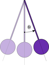
To get an idea of how linear stability theory works, let's look at an
example - the pendulum. Not the perfect, ideal pendulum you might
meet in A-level mechanics, but a real pendulum with its weight
spread out along its length and a bit of air resistance slowing it
down. Now suppose our pendulum is in a steady state - it's not
moving and we're not holding it. What position must it be in?
You probably guessed that it must be at the bottom of its circle of
possible positions. This hanging position is called a stable
equilibrium. The word equilibrium simply means balance. Now say the
pivot moves very slightly. This sort of "noise" - maybe vibration
from traffic outside, or a breeze blowing through - is impossible to
avoid in real life. Our pendulum may swing a little, but as air
resistance damps the motion it will return to rest. That fact is what
defines our equilibrium as stable.
In fact there is another position where in theory the pendulum can be
in equilibrium - at the top of its circle of possible positions. It
will only have gravity and the force at the pivot acting on it, and
these are both vertical, so what would make it fall one way or the
other? It is possible to balance a pendulum "upside down" - but it
takes a lot of effort, as you'll know if you've ever tried to balance
a pencil on your finger. The reason is that this position is an
unstable equilibrium. Going back to the pendulum, if the pivot
moves very slightly, the pendulum will tilt very slightly one way or
the other. Then gravity pulls it further in that direction, and very
quickly the pendulum is a long way away from the equilibrium
point. Because we can't eliminate noise in real life, you would never
expect to see a pendulum balancing heavy end up.

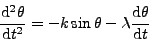
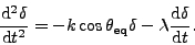
 is the angle measured from the bottom of the swing,
 is a positive constant related to the shape and length of the
pendulum, and
is a positive constant related to the shape and length of the
pendulum, and  is another positive constant relating to the
amount of air resistance.
is another positive constant relating to the
amount of air resistance. and
and


 and
and  : the bottom and top positions.
 to our system.
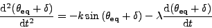
 to expand this:

 and
and  , and also
 , so
, so
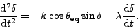
 or smaller. When we've finished,
our system is linear because every term contains exactly one
power of
or smaller. When we've finished,
our system is linear because every term contains exactly one
power of  or
or  .
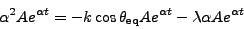
. , so we get:
 , and look to see which values of
  work.
work.
 and
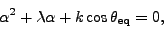
and  so our equation is
 and rearranging,
 and
and
 so
so
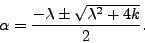
 is
bigger than
is
bigger than  , the square
root is bigger than
, the square
root is bigger than  so
so  and
and
 is less than
 means both the solutions are negative.
The "kick" dies away exponentially.
means both the solutions are negative.
The "kick" dies away exponentially.