Scaling

Introduction

At this point you should have a reflection file created by Mosflm called mosflm.mtz You can view this by using the ccp4 utility mtzdump. To do this type:

setccp4

mtzdump hklin mosflm.mtz

and then after all the program information comes up type:

go

After the header section, you will see that the file consists of a list of "batches" with each batch corresponding to one of your data images. This is because Mosflm records reflections per image. The next step in data processing is to combine all the reflections, look to see which are equivalent between the different images, and scale everything together. To do this five programs are used:

• matthews_coef calculates the number of asymmetric units in your unit cell.
• sortmtz sorts the reflections, and can be used to combine different mtz files.
• scala scales all the equivalent reflections together and generates statistics indicating the quality of your data.
• truncate converts any negative intensities to positive and then converts them into mean amplitudes putting them on an approximate absolute scale using a Wilson plot.
• freerflag flags a fraction of your reflections for use as your "R free" set during later refinement.

With the introduction of the CCP4i GUI all of these programs can be run in just two steps. However, before you can do this you need to set up the CCP4i GUI:

CCP4i Graphical User Interface (GUI)

I find it good practice to create a new directory called ccp4 (mkdir ccp4), go into this directory and then type:

setccp4

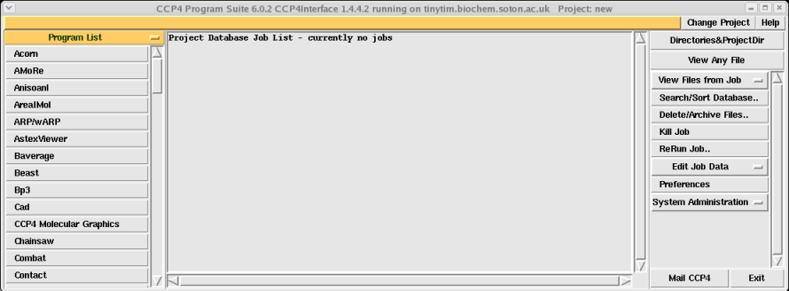
ccp4i

Click OK when it asks if you want to set up a new ccp4 database, and after a couple seconds you should see the following window:

You will need to set up a new project which you can do by clicking on the "Directories&ProjectDir" button on the top right, and then on the next screen click "Add project" (on the right), type in a short reference name in the box next to the word "Project" and then give it the directory path of your new ccp4 directory created above (something like /home/simon/myprotein/ccp4/). IMPORTANT: you then need to select your new project by clicking on the tab in the middle of the screen next to the words "Project for this session of CCP4Interface" and selecting the name of your new project. Once you've done this click on "Apply&Exit" on the bottom left of the screen.

Calculating the Matthews coefficient (solvent content)

You need to calculate the number of asymmetric units in your unit cell for use later on in scaling. You can do this by calculating the solvent content. On average protein crystals should have a solvent content of around 43%, which equates to a Matthews coefficient of between 1.7 and 3.5 cubic A/Da.

On the program list to the left of the screen scroll down and select "Matthews_coef". (If the program list is not available click on the yellow tab with the minus sign on the left of the screen and select "Program List" on the bottom of the drop-down menu). Once you have opened Matthews_coef you should see the following window:

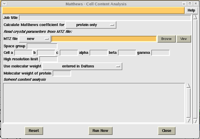
You can enter an arbitrary job title, and then need to select your mosflm.mtz file using the "Browse" button to the right of the MTZ file box. When you load your file the program will automatically fill in the space group, and cell boxes. Next you need to enter the molecular weight of your protein in Dalton's and then click the "Run Now" button at the bottom, middle of the window. After a couple seconds you should see something like this:

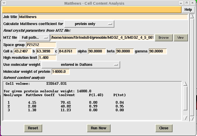
To interpret your results you need to look down the "%solvent" column and choose the line with a solvent content closest to 43%. In the above example this equates to 2 molecules per asymmetric unit (i.e. in this case two 14,000Da monomers in the asymmetric unit). Write down this value and then click the "Close" button.

Scaling

Click on the "Program List" tab on the top left of the CCP4i GUI and select "Data Reduction". Next select "Scale and Merge Intensities" which should give you the following window:

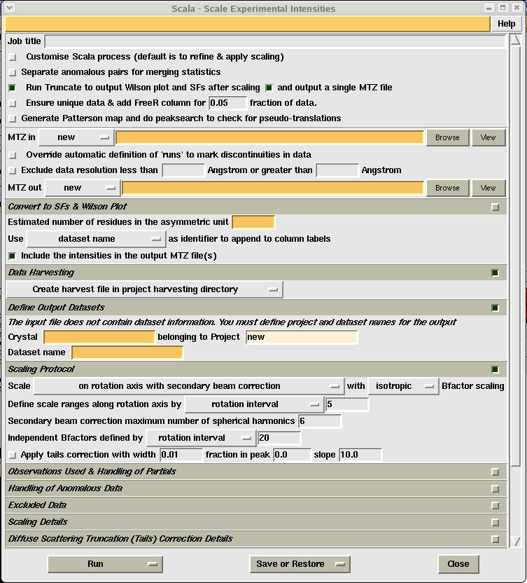
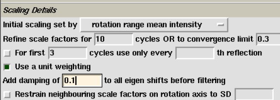
In general the orange boxes are the ones you HAVE to fill in, the little green squares show a selected option, and the little grey squares an unselected option. You can access extra option by clicking on the little squares on the right of the different menu options, however all the options necessary for running the program should be visible straight away.

To run the program:

1. Give the job a name in the "Job Title" bar
2. Click on the grey box to the left of the words "Ensure unique data & add FreeR column for 0.05 fraction of data" (this is normally OK although if you have very high or low resolution data you might want to fiddle with this to ensure you pick about 2000 reflections for your free R set).
3. Using the "Browse" button select your mosflm.mtz file in the "MTZ in" box.
4. Type in what you would like your output file to be called in the "MTZ out" box (I suggest mosflm_scala.mtz). If you like you can limit the resolution range by selecting the line above this box and manually setting your resolution limits.
5. In the "Estimated number of molecules in the asymmetric unit box" enter the number you calculated in Matthews_coef.
6. You can enter an arbitrary reference in the "Crystal" box (i.e. Crystal1) and similarly in the "Dataset" box (i.e. Dataset1).

Once you have filled all these in click "Run" and then from the drop-down menu click "Run&View Com File". This should give you the following window:

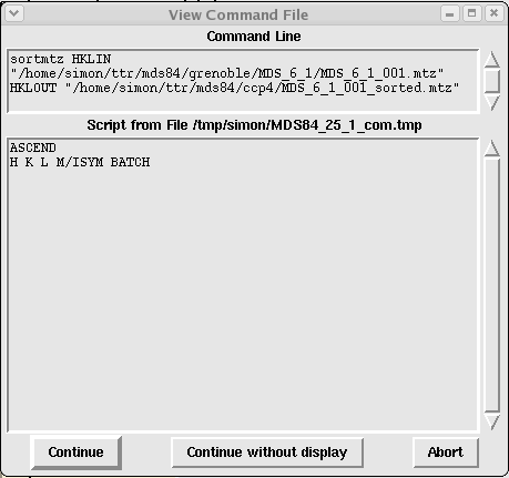
Although not particularly informative in this case, this is the box that displays all the commands necessary to run CCP4 programs. It is normally well worth being aware of these commands whenever you run anything in CCP4i as when things go wrong, this is normally where you can change them. Click "Continue" to run the job.

Once the job is running you can close the scaling input window (click "Close") and you should now see your job listed as "Running" in the main CCP4i window. This may take between five and ten minutes, again depending on the speed of your computer and how big your dataset is.

Scaling Results

When the job has finished (it will say "Finished" in the CCP4i window) highlight the job by clicking on it, and then click on the "View Files from Job" button on the right of the screen, and then click on "View log file". This should open a new window which you should then maximize. Scroll just over half-way down the log file (it is very long!) until you find the red table that looks like this:

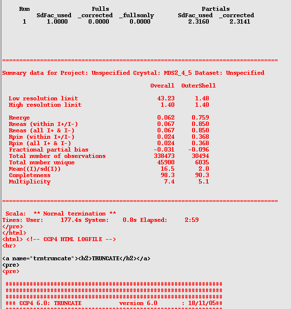
Ideally you will want your overall "Rmerge" to be below 0.2, and your "Mean((I)/sd(I))" to be 2 for the outer shell, and over 10 overall. You also should have a "Completeness" of over 90% overall, and a multiplicity generally higher than 2.

A little aside:

There are quite a few different opinions as to what constitutes good data at this stage. My feeling is that ultimately you need data that will give you an accurate refinement of your structure. I have found that you *can* make a couple compromises at this stage, however if you are going to compromise be prepared to argue for WHY you have compromised! Below are a couple examples with my attempt at a rationale:

If your Mean((I)/sd(I)) is below 2 in your outer shell you will need to reduce the resolution of your data. If it is around 2 I personally would leave it, however, some people might question the wisdom of this if you have a very high Rmerge (in this case 0.759). My counter-argument would be that there are still 6035 recorded spots with over 90% completeness in this shell and a relatively high multiplicity of 5.1. Thus I think you would be throwing out quite a lot of good data if you reduced the resolution.

If you are still not sure you can scroll back up the log file until you find the following tables (just above half-way):

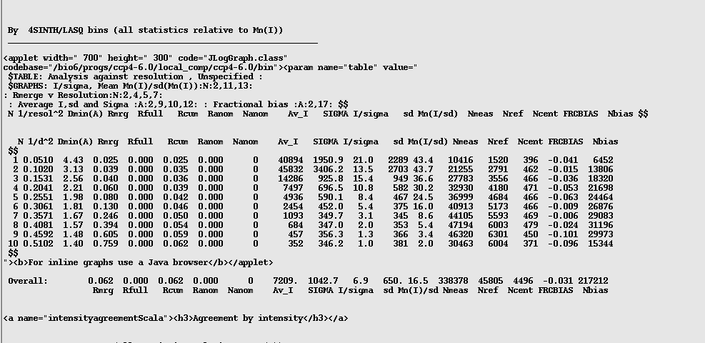
In this table you want to check to see if the quality of your data drops off suddenly as the resolution increases. You can follow this by looking at the "Mn(I/sd)" column and also the "Rmrg" column. With this data you can see the Rmrg doubles between 1.57 and 1.48A, which for some people might be good cause to cut the data at 1.57A.

Next have a look at the following table, two below the previous table:

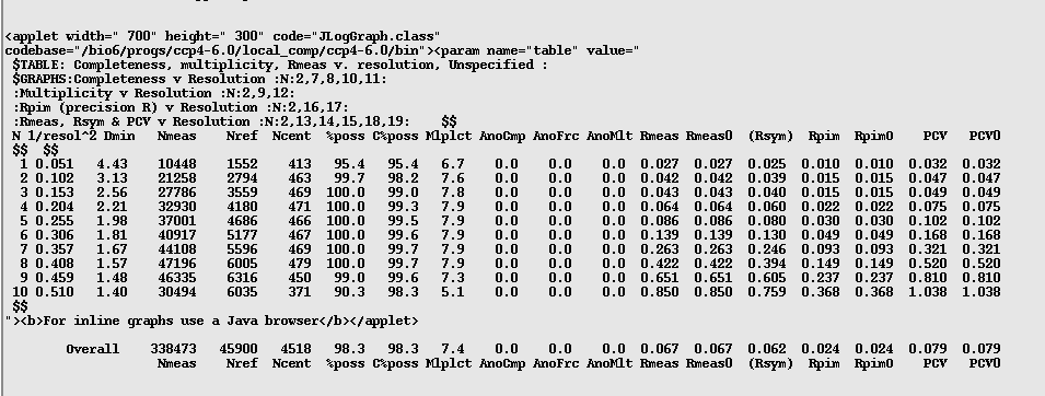
This table shows number of reflections, completeness and multiplicity (amongst a couple other things) across the different resolution shells. Again you want to look to see if your data drops off significantly at higher resolutions. In this example there is a drop between 1.48 and 1.4A, however the overall values for completeness (%poss), multiplicity (Mlplct) and Rmeas all look OK to me.

Finally, you need to check the Wilson plot outputted from the "Truncate" part of the program. This is located about two thirds of the way down the log file, and should look something like this:

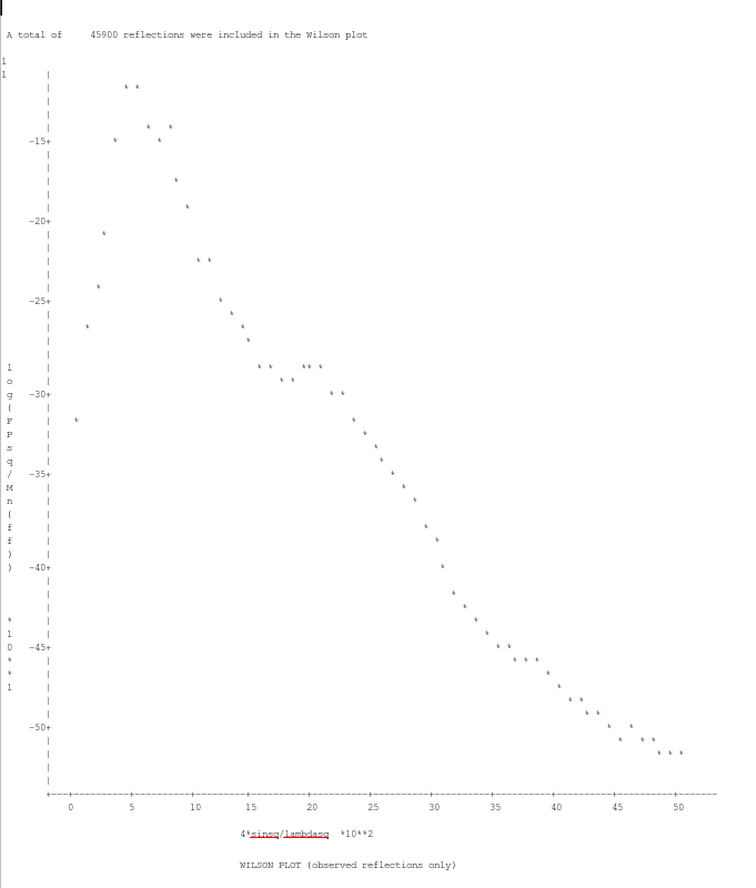
This essentially shows a tail off in spot intensity as resolution increases. You just need to make sure you have a roughly linear relationship at higher resolution as above (don't worry about the bump in the lower resolution data, this is to do with a bias in how the scaling is performed).

If you would like to see more graphs and analysis you can close your log file and then, making sure your scaling job is highlighted, click on "View Files from Job" and then "View Log Graphs". If you click through the options you will find all the above tables represented in graphical format such as:

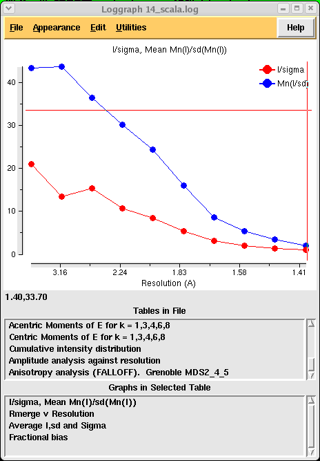
You are of course free to read up on what all this means on the CCP4 website!

Assuming you are satisfied with the quality of your data, you will now have a scaled and merged dataset called mosflm_scala.mtz which you can look at using mtzdump (mtzdump hklin mosflm_scala.mtz). This time, instead of a list of batches you will have a list of reflections, and the file itself should be about ten time smaller than the mtz file that came out of Mosflm (in the above example, 3Mb rather than 80Mb).

If you need to go back and reduce your resolution you can do this by highlighting your earlier scaling job in the CCP4i GUI and then clicking on "ReRun Job". If your statistics are substantially worse than I have described above you probably have a space-group problem. In this case I would go back to Mosflm and play around with the autoindexing a little more.

SCALA errors and tips:

• If your scala job fails with the warning: **** ERROR: damping has failed to prevent negative scale factors **** the scales are varying so much across your images that some of them are coming out negative. Try adding a damping of say 0.1 to the scale factors e.g.

Back to Toolbox