Performing experiments using FTFs
Predicting a grammatical variable from a socio-linguistic one, continued
How big is the effect?
A statistically significant result could be small or large. As we have seen, significance just tells us that a result is unlikely to be due to chance. Moreover, in order to generalise from the significant result, the experimental sample should approximate to a random sample from a specified population of utterances (e.g., in the case of ICE-GB, the population might be 1990s British English, spoken and written).
If the result is significant, it doesn’t mean that the effect is large. Below, we discuss four different measures of effect size. These are
![]() relative size (proportion, sample probability)
including margins of error
relative size (proportion, sample probability)
including margins of error
![]() relative swing (change in proportion)
relative swing (change in proportion)
![]() chi-square contribution, and
chi-square contribution, and
![]() Cramer’s phi association measure.
Cramer’s phi association measure.
Relative size
A useful indication of the size of the effect is the proportion of cases in a category, i.e., the sample probability that a specific outcome is chosen (e.g., who over whom), given a particular value of the independent variable (in the example, text category).
dependent
variable |
|||||
dv |
... |
TOTAL |
|||
independent variable |
iv |
O(dv,
iv) |
TOTAL(iv) |
||
... |
|||||
TOTAL |
TOTAL(dv) |
TOTAL |
|||
A schematic contingency table and values relevant to a particular point [dv, iv]
In the previous example, 150 out of 200 cases (75%) found in the spoken category are who, with 60 out of 100 cases (60%) in the written. If iv represents the different values of the independent variable, and dv the values of the DV (a particular query), O(dv, iv) represents the observed value (a cell in the table), so the formula is
probability pr(dv | iv) = O(dv, iv)/TOTAL(iv).
Thus
probability pr(who | spoken) = O(who, spoken)/TOTAL(spoken) = 150/200 = 0.75.
Probabilities are a normalised way of viewing frequencies (they are between 0 and 1 and, for a fully enumerated set of alternatives, must sum to 1). This probability is the sample probability of the experiment, that is, if the sample were truly representative of the population, this would be the likelihood that a particular dependent value was chosen if a specific value of the independent variable was selected.
Margins of error
As we noted, the probability quoted above is a probability estimate based on the corpus sample. Were we to reproduce the experiment with a different corpus sample taken from the same population of English utterances, we might not get the same result. Consequently, when we make an estimate like this it is useful to also calculate the probabilistic margin of error or confidence interval. This is the likely range of probability values.

|
|||||||||||||||||||||||||||||||||||||||||||||
| critical
values of z (from Wikipedia) |
|||||||||||||||||||||||||||||||||||||||||||||
The table on the right lists critical values of z for some common error points. The way to read the table on the right is to pick the relevant percentage point and read off the critical value of z. Thus 95% of cases in a normal distribution fall within 1.95996 standard deviations of the mean.
The standard deviation of the Binomial distribution is calculated by the following formula:
standard deviation s = √np(1-p),
where p = pr(dv | iv) and n = TOTAL(iv).
However, this is the standard deviation for the actual observed frequency. To estimate the error margin of the observed probability, the standard deviation must be divided by the total number of cases n. This formula can then be rewritten as
probabilistic standard deviation s(p) = √(p(1-p) / n).
Note that as n, the number of cases, increases, the probabilistic standard deviation falls (the error margin shrinks).
In the above example, s(p) = √(0.75 x 0.25 / 200) = 0.0306. The Binomial confidence interval (at the 0.05 error level) is therefore z(crit) x s(p), so with z(crit) = 1.95996 the confidence interval is 0.06. We can write this as the probability pr(who | spoken) = 0.75 ±0.06.
A variation on this method is Wilson's score interval method. This rather less well-known method compensates for so-called 'floor' and 'ceiling' effects in skewed distributions where p is close to 0 or 1. The problem is illustrated by the figure below. Note that p cannot be less than zero, so the Normal distribution, represented by the dotted line, cannot be a realistic pattern of the expected distribution. Instead the distribution is skewed towards the centre of the range (p=0.5).

We have an unequal confidence interval (w-, w+) which is computed by the following formula.
Wilson score interval (w-, w+) = [p + z²/n ± z √(p(1-p)/n + z²/4n)] / [1 + z²/n].
See also Binomial distributions, probability and Wilson’s confidence interval, Wallis (2009).
Relative swing
We can use the relative size to calculate the percentage swing, or change in the probability towards or away from a particular value of the independent variable depending on the grammatical choice.
Depending on the experimental design, you may be interested in
- a change from one value of a variable to another (e.g. a change over time) or
- the effect of selecting a value, in which case you might measure the swing from a central point.
Here we consider the second of these. The first is discussed in Wallis (2010), z-squared: the origin and use of χ².
In our invented example, 150 out of 200 instances found in the spoken subcorpus are who (75%) compared to the remaining 50 cases (25%), which are whom. Suppose that we calculate the swing towards who in the spoken category. As before, we will consider the case where iv is spoken and dv is who.
probability pr(dv | iv) = O(dv, iv)/TOTAL(iv).
The swing is calculated by the difference between this value and the prior probability for the value, i.e., 210 out of 300. This is written:
prior probability pr(dv) = TOTAL(dv)/TOTAL, and
relative swing(dv, iv) = pr(dv | iv) - pr(dv),
where TOTAL is the grand total. This gives us a percentage swing towards spoken for who as follows:
swing(who, spoken) = pr(who | spoken) - pr(who) = 0.75-0.7 = 0.05,
which we could write as +5%.
Margins of error for relative swing
Note, again, that this makes the naive assumption that the sample is representative of the population.
To calculate the confidence interval of two uncorrelated observations we use the Bienaymé formula, or “sum of variances rule”. This states that the variance of the difference between the variables is the sum of the variances, so total s² = s1² + s2².
standard deviation s = √(s(p)(who | spoken)² + s(p)(who)²).
Above we calculated s(p)(who | spoken) = 0.0306. To calculate s(p)(who), we substitute p = pr(who) = 0.7 and n = TOTAL = 300 into the equation for the Binomial standard deviation. In the example, s(p) = √(0.7 x 0.3 / 300) = 0.0265. Substituting, we get s = √(0.0306² + 0.0265²) = 0.0405. The standard error is then 1.95996 x 0.0405 = 0.0793.
We can present this as a swing of 0.05±0.0793, or between -3% and +13%. The interval crosses the zero point, which means that we cannot say that there is a significant swing toward who in the spoken data. (We already shown that who is not significantly selected using a goodness of fit test here). Clearly this is a large confidence interval, but it can be reduced if more data is forthcoming (i.e. as n increases the probabilistic standard deviation falls).
Chi-square contribution
As we have commented, relative size and swing do not take into account the margin of error introduced by the fact that we are calculating from a sample. We need to try to take this into account, particularly if the sample is quite small (at a conservative estimate, where there are less than 20 cases in a single cell or less than 100 cases in total). One way to do this is, as we saw above, to compute the Binomial confidence interval for each case.
Another approach, based on the chi-square contribution, tells us which independent variable values contribute the most to a particular outcome.
Suppose we consider, not the significance test itself, but the individual contribution made towards the total chi-square by each value. We return to our invented example to illustrate the point.
| DV (choice = whom over who) | |||
| IV (text category) | observed O whom |
expected E TOTAL/SF |
chi-square contribution |
| spoken | 50 | 60 | 1.667 |
| written | 40 | 30 | 3.333 |
| TOTAL | 90 | 90 | 5.000 |
Recall that
chi-square χ² = Σ(E-O)²/E, so
chi-square contribution = (E-O)²/E,
where O = O(dv, iv) and E = TOTAL(iv) x TOTAL(dv)/TOTAL (this fraction is the scale factor SF).
If an individual contribution is high, it is either because the expected value is low or the difference between the observed and the expected is reasonably high. If the independent variable has more than two values, you might like to consider whether the distinction between a specific value and all the others would be significant. You can do this with a simple mini-χ²: the “x vs. the world” chi-square. This is a 2 x 2 chi-square which consists of the chi-square contribution for a particular value plus its complement, which is defined as
chi-square contribution complement = (E-O)²/(TOTAL(iv)-E).
You can compare this mini-χ² with a critical value for χ² (df = 1) to ascertain whether a value is individually significant. (Tip: if the chi-square contribution alone surpasses the critical value, you don’t have to work out the complement!)
Cramér’s phi
The problem with chi-square as a measure of association is that it is (a) proportional to the square of the size of the dataset and (b) unscaled. It is difficult to compare chi-square values between different samples. “Cramér’s phi” is a probabilistic measure that essentially corrects for this.
φ = √χ²/(TOTAL x (k-1))
where χ² is the total from the table, k is the row or column width, whichever is lower.
This formula derives a single 'size of effect' measure for any contingency table.
It doesn't work for goodness of fit tests to measure change across a single value. However Wallis (2010) gives a method for calculating a goodness of fit φ which is comparable to percentage swing, but does not suffer from some of its defects.
As you can see, these measures may be used both to measure the size of the overall effect and indicate specific values that you might wish to focus in on and subdivide further.
Common problems
The following problems are discussed below:
![]() have we incorrectly specified the null hypothesis?
have we incorrectly specified the null hypothesis?
![]() have we listed all the relevant values?
have we listed all the relevant values?
![]() are we really dealing with the same linguistic choice?
are we really dealing with the same linguistic choice?
![]() have we counted the same thing twice?
have we counted the same thing twice?
![]() how can we investigate how two grammatical variables
interact?
how can we investigate how two grammatical variables
interact?
More complex problems are discussed on the final
page:
![]() have we effectively captured the aspect of the annotation
we require?
have we effectively captured the aspect of the annotation
we require?
![]() can we tell if cases overlap
one another by examining the corpus?
can we tell if cases overlap
one another by examining the corpus?
Problem: have we specified the null hypothesis incorrectly?
If you followed the steps in the basic example above, you should have no problem. However, often researchers make the assumption that the expected distribution is just based on the quantity of material in each subcorpus. In a lexical or tagged corpus it can be more difficult to calculate an expected distribution because it might involve listing a large number of possible alternatives.
For example, suppose we compare the frequency of the modal verb “may” in a series of subcorpora, with the quantity of material in each one. Appropriately scaled, this could be quoted as the frequency ‘per million words’, ‘per thousand words’, etc.
However, there is an obvious problem with this: what if we found that “may” appeared more frequently than expected in, say, formal writing. This does not tell us if either
- there are more uses of modals in formal writing, or
- there are more uses of modal “may” than other modal alternatives (e.g., “can”) in formal writing.
Variation that we find may be due to the variation in the distribution of an entire group (type a), in which case the explanation should really be more general; or due to variation within the group (type b), variation that may be hidden if we simply compare the distribution of cases with the overall distribution of words.
This means that we should avoid using the quantity of material in a corpus to estimate the expected frequency. In grammar, the possibility of a particular linguistic expression is dependent on whether the expression was feasible in the first place, and this feasibility may also vary with the independent variable.
Instead of using the distribution of corpus material, we base the expected distribution on a general case that identifies when the possibility of variation arises. There are two ways of doing this: top-down, or, as in the previous example, bottom-up.
- Bottom-up. List the outcomes that we are interested in and then define the expected distribution by adding together each of these outcomes' distributions. This is what we did in our “who vs. whom” experiment.
- Top-down. Define the case distribution first, and then subdivide it fully, listing all possible alternatives. On the next page we illustrate this with some examples exploring grammatical interaction.
In summary, the useful null hypothesis is that the outcome does not vary when the choice arises in the first place rather than that it does not vary in proportion to the amount of material in the corpus.
Finally, note that you can, of course, work in both directions within the same experiment. In the following example we define who vs. whom and work from the bottom, up; then we define a which/what+N group and subdivide this (i.e., we work top down).
Problem: have we listed all the relevant values?
When you fail to list or enumerate all possible outcomes of a particular type, it also affects the conclusions that you can draw.
In the worked example we suggested that there were two possible alternative outcomes, who and whom. The DV is defined as one or the other of these. Note that in the formal outline we wrote that the row total was an expression like ‘a and (x or y or...)’ rather than just ‘a’ - there might be other values that are not included in the choice of ‘(x or y or...)’.
If we fail to consider all plausible outcomes our results may be too specific to be theoretically interesting (see the discussion on meaning) and may be more likely to be due to an artefact of the annotation.
Sometimes we may want to add other alternatives while prioritising certain grammatical distinctions over others. To do this, we group alternatives hierarchically to form an outcome taxonomy.
If two outcomes are subtly different from one another, but quite distinct from a third (e.g., who vs. whom vs. which/what+N constructions, we might like to consider two different tables and sets of tests:
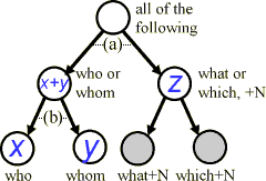
- to compare the first two aggregated together vs. the third (when do we use who or whom?), and
- to focus on the difference between the first two (when do we prefer who over whom?).
The contingency table should be split into two as follows.
| original: x vs. y vs. z |
(a) (x
or y) vs. z |
(b) x
vs. y |
||||||||||||||||||||||||||||||||||||||||||||||||||||||||||||||||
|
|
|
||||||||||||||||||||||||||||||||||||||||||||||||||||||||||||||||
We may also choose to further subdivide the which/what+N constructions (in the figure: greyed, right).
Problem: are we really dealing with the same linguistic choice?
One advantage of working from the bottom, up, rather than from the top, down, is that this method encourages you to think about the specifics of each linguistic choice. Our assumption has been that who and whom are interchangeable, i.e., any time a speaker or writer uses one expression the other could equally be substituted. Likewise, in the illustration above, we effectively assumed that in all cases where who or whom were used, a which/what+N expression could be substituted, and vice-versa. But sometimes you need to check sentences in the corpus to be sure.
This is a particular problem if you want to look at a phenomenon that is not represented in a corpus. For example, in ICE-GB, particular sub-types of modals are not labelled. Suppose we wished to contrast deontic (permissive) may with deontic can, and then compare these with other ways of expressing permission. We don’t want deontic may to be confused with other types of modal may, because these other types do not express the same linguistic choice. The solution is to first classify the modals manually (effectively by performing additional annotation). This will be possible through the use of ‘selection lists’ in ICECUP 3.1.
![]() This problem is related to issues arising from the annotation.
This problem is related to issues arising from the annotation.
Problem: have we counted the same thing twice?
If you include cases that are not structurally independent from one another you flout one of the requirements of the statistical test. You cannot count the same thing twice.
The problem arises because a corpus is not like a regular database and ‘cases’ interact with one another.
There are several ways in which this “bunching” problem can arise. We have listed these from the most grammatically explicit to the most incidental.
- Matches fully overlap one another. We discussed this in the context of matching the corpus (see here). The only aspect of this matching that can be said to be independent is that different nodes refer to different parts of the same tree. If you avoid using unordered relationships in FTFs, this will not happen.
- Matches partially overlap one another, i.e., part of one FTF coincides with part of another. There are two distinct types of partial overlap: where the overlapping node(s) in the tree are the same in the FTF, or different. The first type can arise with eventual relationships in FTFs, the second can only occur if two nodes in an FTF can match the same constituent in a tree (see detecting case overlap here).
- One match can dominate, or subsume another, for example, a clause within a clause.
- Alternatively a match might be related to another via a simple construction, e.g., co-ordination.
- The construction may be repeated by the same speaker (possibly in the same utterance) or replicated by another speaker.
If you are using ICECUP to perform experiments, you can ‘thin out’ the results of searches by defining a 'random sample' and then applying it to each FTF. However, this thins out sentences, not matching cases. If several cases co-exist in the same sentence and the sentences are included they will all be included. Moreover, since this will mean that the number of cases will fall, the likelihood that an experiment is affected by the limited independence of cases will increase.
We should put this in some kind of numerical context: if you are looking at (say) thirty thousand clauses, it is unlikely that a small degree of bunching will affect the significance of the result. If, on the other hand, if you are looking at a relatively infrequent item (say, in double figures) and when you inspect the cases you find that many of these are co-ordinated with each other, you may want to eliminate these co-ordinated items, either by limiting the FTF or by subtracting the results of a new FTF that counts the number of additional co-ordinated terms for each outcome.
The ideal solution would be for the search software to identify potential problems in the sampling process and discount interacting cases in some way. We have been investigating this problem (as part of a process called knowledge discovery in corpora), and hopefully, we can support this in a future software release. Until then, however, you should bear our comments above in mind.
Problem: how can we investigate how two grammatical variables interact?
Propositional (drag and drop) logic, which we have used up to now, works fine for a socio-linguistic predictor combined with an FTF. This is because a ‘case’ in socio-linguistic terms consists of a set of text units. But each text unit can contain several cases of the same grammatical construct. What if we want to study the interaction between two aspects of a single grammatical construct?
We cannot merely compute intersections to collect the statistics. We have to be sure that the table correctly summarises distinct classes of matching cases in the corpus. How do we do that?
![]() This is the question we turn to next.
This is the question we turn to next.
![]()
FTF home pages by Sean Wallis
and Gerry
Nelson.
Comments/questions to s.wallis@ucl.ac.uk.
This page last modified 28 January, 2021 by Survey Web Administrator.