Performing experiments using FTFs
Predicting a grammatical variable from a socio-linguistic one
The basic approach: constructing a contingency table
On the previous page we discussed what a hypothesis was and introduced the idea of an experiment that was designed to test this hypothesis. In order to evaluate the hypothesis, we perform a series of searches in the corpora and then construct a table, called a contingency table, which summarises the data. An outline is given below. The table helps us to collect and organise our data in order to perform a χ² (chi-square) significance test.
Later in these pages we will worry about experiments that test whether one grammatical variable could contribute toward variation in another. For now we will confine ourselves to experiments that consist of studying whether socio-linguistic variables affect grammatical preferences. Thus, in our example, we were interested in finding out whether a socio-linguistic variable (text category) affects the grammatical ‘choice’ of using “whom” rather than “who”.
We will first outline the basic approach.
Recall that an experiment tests the hypothesis that "the IV affects the DV" (the independent variable affects the dependent one).
- We construct a contingency table as follows, filling
in the cells we have coloured in green by searching the corpus.
Using ICECUP, we can perform
a series of FTF queries, one for each grammatical outcome (DV = x,
y, ...). We then calculate the overlap, or ‘intersection’,
between each of the FTF queries and each value of the socio-linguistic
variable (IV = a, b,...) (In
ICECUP, you can employ drag
and drop logic to compute the intersection.)
We can express a general contingency table algebraically as follows. Naturally, each total is the sum of the preceding row or column, and ‘a and x’ means the intersection of ‘IV = a’ with ‘DV = x’.
| dependent variable (grammatical choice) | |||||
| DV = x | DV = y | ... | TOTAL | ||
| independent
variable (sociolinguistic context) |
IV = a | a and x | a and y | a and (x or y or...) |
|
| IV = b | b and x | b and y | b and (x or y or...) |
||
| ... | |||||
| TOTAL | (a or b or ...) and x | (a or b or ...) and y | (a or b
or ...) and (x or y or...) |
||
A general contingency table (DV x IV)
-
We want to find out whether the independent variable affects the value of the dependent variable, i.e. the choice of the grammatical construction. To do this we contrast the distribution of each grammatical choice with the distribution that would be expected if it were unaffected by the IV.
- We can set up a simple chi-square test (written χ²)
for the outcome DV = x. If this chi-square
is significant it would mean that the value of the independent
variable appears to affect the choice of outcome x. (Strictly,
the null hypothesis - that it is unaffected - is not supported.)
The chi-square compares an observed distribution for DV = x
with an expected distribution based on the total (DV
= <any>).
Important reminder: do not assume that the total (which is proportional to the likelihood of the choice occurring in the first place) is distributed in proportion to the quantity of the material in the corpus. This is an all-too-common mistake. For more on this, see the discussion on relative frequency on the previous page or, for the experimental conclusions of this argument, the next page.
dependent
variable (grammatical choice) |
|||||
DV
= x |
DV
= y |
... | TOTAL |
||
independent
variable |
IV
= a |
a
and x |
a and y |
a
and (x or y or...) |
|
IV
= b |
b
and x |
b and y |
b
and (x or y or...) |
||
... |
|||||
observed |
expected |
||||
Observed and expected distributions for DV = x in the contingency table
- Before performing the test, the expected distribution should be scaled so that it sums to the same as the observed distribution. To calculate the scale factor, divide the column totals by one another: SF = TOTAL(obs) / TOTAL(exp). To scale the expected column, multiply all values by SF.
We can perform the chi-square for any other choice: DV = y, etc., and for the entire table (see below). All observed distributions are compared against all expected distributions in a single chi-square.
Our example, with invented data
Suppose our IV is spoken or written, i.e., the simplest subdivision of text category, and we are interested in a grammatical choice: who vs. whom. The table now looks like this.
| DV (use of “whom” over “who”) | ||||
| who | whom | TOTAL | ||
| IV (text category) | spoken | who in spoken | whom in spoken | (who + whom) in spoken |
| written | who in written | whom in written | (who + whom) in written | |
| TOTAL | who in (spoken + written) | whom in (spoken + written) | (who + whom) in (spoken + written) | |
Constructing a table for our example experiment
This is a simple 2x2 contingency table, i.e., both variables have two possibilities. By performing the necessary searches we obtain the four central figures, then sum the rows and columns. We then apply this data to a chi-square test. Instead of performing the experiment, for clarity we’ll demonstrate the idea with some invented numbers.
grammatical
choice |
||||
who |
whom |
TOTAL |
||
text category |
spoken |
150 |
50 |
200 |
written |
60 |
40 |
100 |
|
TOTAL |
210 |
90 |
300 |
|
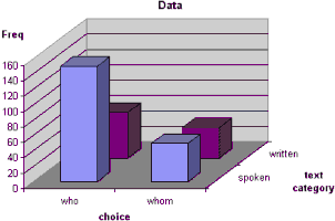
A simple (invented) example of a contingency table
In order to visualise the distribution we can plot it in the form of a simple bar chart. The vertical represents the frequency, i.e. number of cases, in each category.
The most striking observation about this data is the large 'spike' for who in the spoken data. But there is also more examples of either who or whom in the spoken part of the corpus.
![]() You can download an Excel
spreadsheet which contains the table above, tables working out
the following χ² tests, and graphs of the distributions.
You can download an Excel
spreadsheet which contains the table above, tables working out
the following χ² tests, and graphs of the distributions.
Having collected the data we can now pose some experimental questions. For example,
Is “whom” chosen in preference significantly more in writing?
It certainly looks like it, just by “eyeballing” the data. According to the table there are 50 cases of “whom” in the spoken sample, compared to 40 in the written subcorpus.
The statistical test, called a goodness of fit χ² test for whom, takes the variation between the total number of cases in spoken and written into account.
The χ² test compares the difference between patterns of observed data, called the observed distribution (labelled ‘O’), and an expected distribution, ‘E’. We calculate E by scaling values in the TOTAL (“who or whom”) column on the right, by the proportion of the sample in each observed column. We then choose a critical value for χ², which must be surpassed by the evaluated χ². You can find a table of critical values for χ² here. There are two cells in the distribution, so the number of degrees of freedom, df = r-1 = 1. By convention, we can accept an error of 1 in 20 (0.05). The following shows the working.
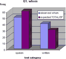
Q1. Is a preference for whom significantly affected by the text category?
| Observed O = {50, 40}, scale factor SF = 90/300 = 0.3, expected E = {200x0.3, 100x0.3} = {60, 30}. Chi-square χ² = Σ(E-O)²/E = 10²/60 + (-10)²/30 = 5.000. |
Note: the expression ‘Σ(E-O)²/E’ is evaluated by summing each separate chi-square contribution (‘(E-O)²/E’) for each pair of values, O, and E. The χ² contribution for the first pair (spoken) is (E-O)²/E = (60-50)²/60 = 10²/60 = 1.667 (approx), the second (written), (30-40)²/30 = (-10)²/30 = 3.333 (approx). |
Chi-square critical value (df = 1, error level p = 0.05) = crit(1, 0.05) = 3.841.
Since χ² > critical value, the result is significant and the null hypothesis, i.e., that whom does not correlate with variation of text category, is rejected.
Answer: Yes. To see possible reasons for the result, see below.

Observed and expected distributions for question 1.
One way of seeing how the test works is to look at a graph comparing the observed and expected distributions. The χ² divides the square of the difference between these two columns with the height of the expected distribution. Here the difference is 10 and the expected distribution is {60, 30}.
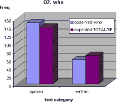
Q2. Is the choice of who over whom significantly affected by the text category?
Observed O = {150, 60},
scale factor SF = 210/300 = 0.7,
expected E = {200x0.7, 100x0.7} = {140, 70}.Chi-square χ² = Σ(E-O)²/E = (-10)²/140 + 10²/70 = 2.142 < crit(1, 0.05) = 3.841.
Since χ² < critical value, the null hypothesis, i.e., that the choice of who does not correlate with variation of text category, cannot be rejected.
Answer: No. Why is this not significant, while the first one was?
Note that the the expected distribution totals are higher but the difference between the two distributions is the same as before (10). As a proportion of the expected distribution, the squared difference is therefore smaller, and the chi-square test accepts that this could be explained by chance.
This is shown in the graph below.
Another way of putting this is that variation in the choice of a relatively infrequent item, like whom, is more important than variation in the choice of a more common one.

Observed and expected distributions for question 2.
Q3. Is the entire grammatical choice (who or whom, but not specifying which) significantly affected by the text category? (NB. This is the most common type of χ² test for homogeneity, and it is how the question is often put in books in experimental design. The number of degrees of freedom, df = (r-1) x (c-1), where r is the number of rows and c the number of columns in the table.)
Observed O = {150, 60, 50, 40},
expected E = {140, 70, 60, 30}.
Chi-square χ² = Σ(E-O)²/E = (-10)²/140 + 10²/70 + 10²/60 + (-10)²/30 = 7.142 > crit(1, 0.05) = 3.841.
Since χ² > critical value, the null hypothesis, i.e., that the grammatical choice does not correlate with variation of text category, is also rejected.
Answer: Yes. We would expect this from the fact that at least one separate outcome is significant. For a 2x2 table, the test simply sums the result of the previous two tests. As a result, this kind of test is weaker than the first two: the conclusion is that there is a significant overall variation without being able to point to where it is.
![]() Further reading: z-squared:
the origin and use of χ² (PDF) 2
x 2 χ² (Excel)
Further reading: z-squared:
the origin and use of χ² (PDF) 2
x 2 χ² (Excel)
What do significant results mean?
A significant result on its own does not mean very much. It simply says that perceived variation is large enough to not be due to chance. Statistical results indicate a correlation, they cannot prove a cause.
A significant result suggests that something systematic is going on which would be reproduced if we were to take similar samples (of text) from the population (of all texts from the same period, authorship, genres, etc., and annotated in the same way). It doesn’t say what is going on. This is the corollary of the argument we made on the previous page regarding the difficulty of proving or disproving a hypothesis.
There is another aspect to significance. If the sample size is very large, almost every apparent variation will be significant (i.e., it would exist in the population). The question is then, it may be significant, but how big is the effect? We consider different measures of effect size on the next page.
Does a significant result prove the experimental hypothesis? Not necessarily...
| Time to play devil’s advocate... |
Possible explanation. The significant result could be an artefact of the annotation. There are at least three different kinds of problem here.
- Circularity. Maybe the result flows from the way that the grammar has been adapted to deal with, say, spoken English. You may find that in practice you were measuring the same thing in two different ways. No wonder the result was significant!
- Inaccurate sampling. It could be due to an imprecise FTF definition, incorrect annotation or poor sampling in the first place (for an example of an annotation weakness, see here). Are all your cases really expressing the same linguistic phenomenon? Are there other cases in the corpus that should have been included? Another possibility is that cases are not strictly independent.
- Poor design. Are all possible values of a variable listed? Are some of the outcomes expressing something linguistically quite distinct to the others? You might want to restructure the experiment to deal with two distinct subgroups (see the example on the next page).
To decide you must inspect the cases and relate the design to a theory.
Possible explanation. The correlation could be a result of a third factor affecting both the DV and the IV separately. This is more likely if the DV and IV are both grammatical. (This is our old friend the root cause.)
Stephen Jay Gould gives the example of the price of petrol correlating with the age of a petrol pump attendant. Just because the petrol price may rise over time, as the attendant ages, it does not mean that the age of the attendant causes the price to rise, or vice-versa!
The central point is that to ascertain the reason for a correlation requires more work. You should inspect the corpus and argue your case. Relate your results to those reported in the literature: if they differ, why do they do so? Play ‘devil’s advocate’ and try to argue against your own results. Dig deeper - try looking at subcategories of each FTF, for example - and anticipate objections.
The beauty of a public corpus and query system is that, provided you report your experiment clearly, everyone has the opportunity of reproducing your results (and possibly raising alternative explanations).
The corpus is a focus for discussion, not a substitute for it.
| Recall the statistical health warning: |
Performing an experiment is not a substitute for thinking
about the research problem. You need to (a) get the
design right and (b) relate the results back to
a linguistic theory. |
As well as detecting a significant difference and even explaining it, it is also useful to be able to measure how big an effect is: a small variation can be significant without being very interesting, while a large variation can indicate that there is something more fundamental going on.
![]() On the next page we discuss different
measures for the size of the effect and a number of potential problems
that researchers have in defining an experiment.
On the next page we discuss different
measures for the size of the effect and a number of potential problems
that researchers have in defining an experiment.
![]() These issues become even more important when we turn to the question
of using one grammatical variable to predict another.
These issues become even more important when we turn to the question
of using one grammatical variable to predict another.
References
Gould, S.J. (1984), The mismeasure of man, London: Penguin.
FTF home pages by Sean Wallis
and Gerry
Nelson.
Comments/questions to s.wallis@ucl.ac.uk.
This page last modified 28 January, 2021 by Survey Web Administrator.

