Gravity, the shape of the Earth, isostasy, moment of inertia

Gravity is one of the four fundamental forces (the others are the electromagnetic, the weak force and the strong force) and probably the least well understood. The basic concepts were formulated by Newton in the 17th century.

These were deductions from Kepler’s Laws of planetary motion.

Johannes Kepler (1571 - 1630), working with data painstakingly collected by Tycho Brahe without the aid of a telescope, developed three laws which described the motion of the planets across the sky.

1. The Law of Orbits: All planets move in elliptical orbits, with the sun at one focus.

2. The Law of Areas: A line that connects a planet to the sun sweeps out equal areas in equal times.

3. The Law of Periods: The square of the period of any planet is proportional to the cube of the semi major axis of its orbit.

Kepler's laws were derived for orbits around the sun, but they apply to satellite orbits as well.

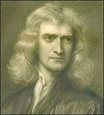
Remember the last £1 note?

Isaac Newton is on the back, and an artist has rendered a planetary diagram next to him.

What's wrong with this picture?

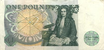
Answer: They've put the sun at the centre of the ellipse!

Many questions remain:

How do masses actually attract each other? 

Are there GRAVITONS?

Is there a “Fifth Force”?

Can the fundamental forces be unified…..

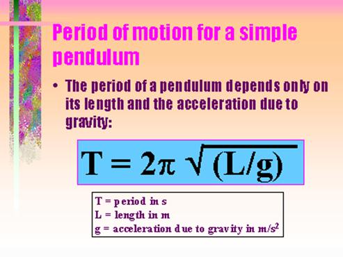
However, gravitational attraction is an everyday experience and its variations provide insights into Earth structure. Early studies used either the periods of oscillation of pendulums or 'deflections of the vertical' measured by observations of fixed stars to measure gravity.

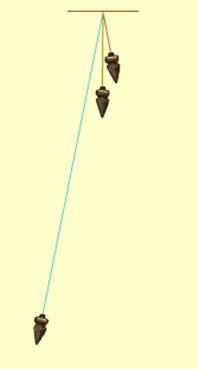
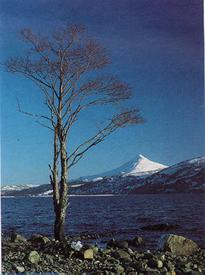
Using Newton’s Laws the Astronomer Royal, Nevil Maskelyne (1732-1811)

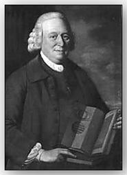
reported in 1755 to the Royal Society an estimate of the mass of the Earth obtained by observations of the deflections on either side of Schiehallion, a mountain of almost perfectly triangular cross-section in the Scottish highlands.

A few years earlier the French scientist Bouguer noted that the gravitational attraction of the Andes was smaller than would have been anticipated from estimates of their very large excess mass. This was the beginning of observational isostasy.

Basic Relations

Described by Newton's Law of Gravitation:-

F = G m₁ m₂ / r² Newtons

F = force acting between two point masses
m₁, m₂ = the masses
r = separation of the two masses
G = Universal gravitational constant = 6.67 x 10^-11 Nm²kg^-2

How do we know G???

The value of G, the universal gravitational constant, was determined by Henry Cavendish  (1731 1810) using the apparatus shown here:

There is a gravitational attraction between the large lead balls M and the small balls m. This results in a slight twisting of the quartz fiber. When the large lead balls are shifted as shown in the upper left of the illustration, the direction of twist is reversed. This movement is amplified and measured by the deflection of a beam of light reflected from the mirror and projected on a ruled scale some distance away. The force corresponding to the twisting of the quartz fiber was previously calibrated using light weights.

Cavendish was terrified of women, and communicated with his female servants by notes.

Newton also found that on Earth:

F=m.g

Where m is a bodies mass, and g is the acceleration due to gravity. But a body of mass m is attracted to the Earth by gravity, with a force:

F = G mM/ R²

Where M is the mass of the Earth, and R is its radius (~6400 km – how do we know this??). It follows that:-

m.g= G.m.M/ R²

g = G.M / R²

The units of g are Newton.kg^-1 (force per unit mass) or (more commonly), m.s^-2 (acceleration). Numerically, these are identical and:

g ~9.81 ms^-2 .

In fact g can be obtained from the period of a pendulum, and so the equation:

g = G.M / R²

is used to determine:

M = 5.9742 × 10²⁴ kilograms

Geologically, the density of earth is very important. If ρ is the average density of the Earth, then

ρ = mass/volume = M / [(4/3)πR³]  = 3M / 4πR³

We can substitute for M using the relationship between it and g, i.e. M = R²g / G. Therefore: 

ρ = 3g / 4πRG

Thus if we know g, R and G, we can calculate ρ. With current values:-

ρ = 5.52 x 10³ kgm^-3

Since most surface rocks have densities in the range 2-3 x 10³kg.m^-3, density must increase with depth in Earth. This has also been confirmed by seismology, since seismic velocities, which are strongly correlated with density, increase with depth.

However, we would also like to monitor lateral density variations. We cannot easily measure density at depth, but it is quite easy to measure g at different places on the surface of the Earth.

How do we Measure Gravity?

• Pendulum

• Mass Dropping

• Gravimeter

• Pendulum

• Period of swing = T

• Mass Dropping

• Distance traveled in time t’ = L

• Both absolute measurements

• Both methods independent of mass, m.

• Both methods should give g ~ 9.81 ms^-2

· Gravimeters

Neither pendulums nor weight drop chambers are suitable for routine field use and instead spring-balance gravity meters are used to estimate changes in g.

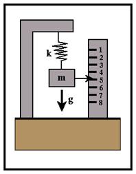
• Gravitational force on a mass is balanced by a force exerted on a stretched spring

• m.g = k.x

x = stretch in spring, k is spring compliance

• Instrument must be stabilised against thermal fluctuations

• Spring made of fused silica - low coefficient of thermal expansion

• Accurate to 1 part in 10⁸

• Common makes - Worden, Lacoste

• Gravimeters expensive and fragile

• Gravimeter measures difference in gravity between 2 locations

• g = cR c = calibration coefficient

Linking such measurements to places where absolute values are known allows us to determine absolute values with gravimeters.

Worden Meter

Gravity and the Shape of the Earth

The variation of g over the surface of the globe is important because it provides information on variations in the shape and internal structure of the Earth.

If we rearrange F = G mM/ R² substituting for M via ρ = mass/volume = M / [(4/3)πR³]  = 3M / 4πR³, we obtain:

g = 4π ρ RG / 3

If the Earth were a perfect sphere of uniform density, g would be constant over its entire surface. But if the Earth deviates from spherical (i.e. if R varies) or if there is a local density anomaly, g will vary.

The Earth is not spherical, but an ellipsoid of revolution i.e. it is flattened at the Poles - this is a rotational effect (see detailed notes).

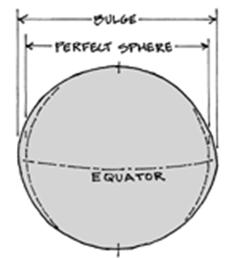
Satellite studies have provided a very accurate measure of ellipticity:-

equatorial radius = 6378 km.

polar radius = 6356.6 km.

Flattening = (6378 - 6356.6 )/ 6378 = 1 / 298.26

Now since g = GM / R², g will be larger where R is smaller. Therefore g at the poles is larger than g at the Equator.

g is also affected by the fact that the Earth rotates and an observer on its surface therefore experiences a centrifugal force.

We can summarise by saying:

(1) If the Earth were a non-rotating perfect sphere, the acceleration due to gravity would be constant.

(2) Because of rotation, the Earth is flattened at poles. This affects g in two ways:-

(a) g at the poles is greater than g at the equator because R at the poles is less than R at the equator.

(b) rotational force at the Earth surface is at right angles to the axis of rotation and proportional to the distance from that axis.  It is therefore zero at the poles and a maximum at the Equator. It acts outwards, reducing g.

The net gravitational force at the surface of Earth is equal to the resultant of the forces due to internal mass and the centrifugal action. If the gravitational force due to M is a = GM / R² and the centrifugal force is c, then the total effective gravitational force is b the vector sum of a and c. However, b does not act towards the centre of Earth, but at right angles to the surface of the elliptical Earth:

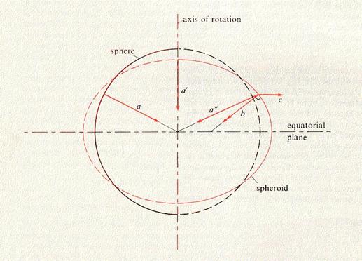
Thus a perfectly homogeneous plastic body will deform until the combination of a and c meets this criterion. In mathematical jargon, the surface of the ellipsoid is an equipotential surface.

The ideal (ellipsoidal) mean sea level surface is called the Earth ellipsoid or (Earth) spheroid.  The gravitational force over the spheroid varies, with a maximum at the poles (where c = 0) and a minimum at the equator (where c is a maximum).

The gravitational acceleration on the surface of the spheroid is given by the International Gravity Formula (IGF).

g = 9.780318 (1 + a sin²(λ) - b sin² (2λ))

where g = sea-level gravitational acceleration on the spheroid and λ = latitude, and a = 0.0053024  and  b = 0.00000587 

g at Equator (lat = 0) = 9.780318 m.s^-2
g at Pole (lat = 90) = 9.832177 m.s^-2

The difference amounts to approximately a half of one percent. The value of the theoretical or normal gravity varies smoothly between the two extremes, but inhomogeneities in the Earth produce shorter wavelength perturbations in the smooth curve.

Variation of gravity with height

At Q (h=0, ie surface)

• g = GM/r²

At P (h=h)

• g = GM/(r+h)²

• g decreases with height

gradient = dg/dh = -2g/R

= 3.086x10^-6 ms^-2/m

= 3.086 gu/m

Units of gravitational acceleration

• 1 gu = 10^-6ms^-2

• 1 mgal = 10^-5 ms^-2

• 10 gu = 1 mgal

Variation of gravity through the Earth

At surface

g = GM/r²

In the Interior, at some radius, r

g(r) = g_MI + g_MO

g_MI = GM_I/r²

g_MO = 0

• g(r) = GM_I/r²

What is M_I?

M_I = (4/3)πr³ρ

· g(r) = (4/3)πrρG

• gravity is zero at Earth’s centre

• In reality the depth curve varies from simple equation because core is much denser than mantle

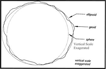
Effect of Inhomogeneities: the Geoid

Large-scale inhomogeneities produce departures of the measured values of g at sea-level from those predicted by the I.G.F. The fact that g does not vary smoothly from equator to pole provides evidence that there are lateral inhomogeneities within the Earth.

Values of g can be determined by surface measurements and by satellite studies.

The real sea level equipotential surface is known as the geoid and has "highs" and "lows" relative to the spheroid. Contours of the geoid give the height, above or below the spheroid, by which sea level actually varies over the Earth's surface.

Sea-level is +54 metres higher in the North Atlantic than predicted by the IGF spheroid, and the maximum departure is -94 m, over India.

The geoid map may be divided into large positive and negative regions (above and below spheroid surface). Most positive features correspond to active magmatic regions:-

e.g. Mid-Atlantic Ridge,The Andes, The Philippines

Negative features are centred over old, inactive ocean basins and continents:-

e.g. Antarctica, Canada, Siberia, India

Major physical undulations (e.g. mountains) are NOT associated with geoid anomalies, and so they must be balanced by deeper seated mass excesses or deficiencies (Isostasy – see below).

It is believed that long wavelength undulations in the geoid reflect the convective system in the mantle, or some other deep phenomena (e.g. undulations on the outer surface of the core).

The problem is complex because of the effects of flow dynamics. Thus, an upwelling should be characterised by low density, which would produce a negative geoid anomaly, but the convective motion deflects the surface and so produces a +ve anomaly.

Crustal Gravity Anomalies

In addition to the global anomalies due to convection, there are smaller scale effects because of crustal inhomogeneities (sedimentary basins, intrusions, etc.).

Their analysis is important in exploration for natural resources, but they also need to be taken into account in global scale investigations and surveys (see also detailed notes).

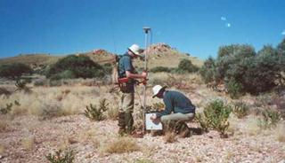
In a gravity survey we measure the difference in gravity between survey points (S) and a reference station (P), using a gravity meter.

Ideally P is either an international gravity reference station or has been linked to such a station by gravity measurements.

Inevitably, the differences will be small and the m.s^-2 is far too large a unit.

Gravity anomalies are therefore measured in gravity units.

1 g.u. = 10^-6 m.s^-2

(An older unit, the milligal, abbreviated as mGal, is still in common use. 1 mGal = 10 g.u.)

Since g is approximately 10 m.s^-2, 1 g.u. is about one ten millionth of the absolute value of gravity at Earth’s surface.

What causes gravity anomalies?

• If ρ₁ ≠ ρ₂ then there is a local mass excess or mass deficiency in the vicinity of the geological body causing a local very small variation in the value of g

• positive anomaly if ρ₂ > ρ₁

• negative anomaly if ρ₂ < ρ₁

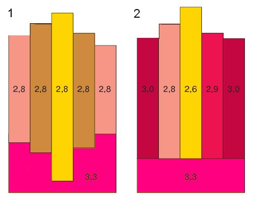
Densities of common rocks and Earth material

• water 1 Mg m^-3 (old units g/cc)

• granite 2.5 => 2.7 Mg m^-3

• limestone 2.66 => 2.7 Mg m^-3

• sandstone 1.8 => 2.7 Mg m^-3

• basalt 2.7 => 3.2 Mg m^-3

• coal 1.2 => 1.5 Mg m^-3

• rock salt 2.1 => 2.5 Mg m^-3

• average density of crust 2.85 Mg m^-3

• average density of mantle 3.3 Mg m^-3

• average density of Earth 5.5 Mg m^-3

Most gravity meters can detect changes in gravity of as little as 0.1 g.u., and need to, as mineable deposits of metals such as copper, lead, zinc, nickel and iron have been discovered on the basis of anomalies of less than 5 g.u.

Underground cavities which could represent hazards to e.g. motorways or airstrips may give rise to effects of only a few tenths of a g.u. .

So a local survey might give:

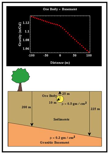
Can fit to background, and get the difference to show up ore body:

Gravity Corrections

The measured value of gravity at a field station might vary from the value at the base station for a variety of reasons, even if there were no crustal or geoid anomalies.

Once the value has been obtained it must be corrected to account for effects such as:-

(1) Latitude differences
(2) Elevation effects
(3) Topographic effects

Any differences that remain after these corrections have been made must be due to real lateral variations in density.

Latitude Correction

We have seen that gravity on the surface of a homogeneous Earth varies from pole to equator because of effect of centrifugal force and polar flattening.

Thus if stations are at different latitudes, we would expect gravity to be different. We use the IGF to describe the latitude effect.

For small N-S distances (up to a few km) the difference in gravity due to latitude at latitude λ is approximately:-

Δg_LAT = 8.1 sin(2 λ) g.u. per km

Free-air Correction

If stations are at different elevations, we would expect gravity to be different because of the different distances to the centre of the Earth.

The effect for a positive height (h) above sea-level is approximately equal to -3.086 g.u./metre, an increase in height produces a decrease in gravity. So g_ground-level > g_highup

Δg_ELEV = -3.086h g.u.

The correction, known as the free-air correction (because, in the derivation, it is assumed that the only material between the station and the reference surface is air), must therefore be positive. So Δg is added to g_high-up to bring it into line with the reference g_ground-level.

Note that if the gravity anomaly is to be measured to within 0.1 g.u., the station elevation (h) must be known to within 3 cm!

Gravity corrections require accurate elevations, and getting these is often the most expensive part of a gravity survey.

Free air gravity survey is often used for marine studies, e.g. Caribbean:

Bouguer Correction

The free-air correction assumes that only air exists between the station and the reference surface.  In reality, a normal gravity station on land will be underlain by rock, of density ρ, which exerts a positive (downwards) gravitational pull.

The Bouguer correction adds to the free-air correction a simple approximation for the effect of this rock column.

We assume that the gravity effect of the real topography can be approximated by the effect of a uniform flat plate, density ρ (in kgm^-3) and thickness h, extending to infinity.

This effect is given by:-

Δg_ROCK = 2π G ρ h = 41.91 x 10^-5ρ h  g.u.

The effect is positive (ie it increases the gravity field) and therefore the correction for the presence of rock must be negative.

For granite ρ is approximately 2670 kg m^-3, and this has been adopted as a “standard” density for the upper crust, giving a correction of -1.118 g.u./metre.

Other densities may be used to suit the local geology, but use of the standard density has the virtue of ensuring compatibility between maps of adjacent areas.

Since the free-air correction is 3.086 g.u./metre, but when the effect of intervening rock is considered the net correction is reduced, so that the net elevation correction, the Bouguer Correction, is about 1.968 g.u./meter, implying that elevations of gravity stations should be known to the nearest 5 cm.

So in this case, again, g_ground-level > g_high-up, but much less than in the free-air case due to the intervening rock.

Terrain Correction

Although the Bouguer correction works surprisingly well, it is inadequate for high precision surveys or for surveys carried out in topographically rugged areas.

If the station is next to a mountain or valley, the mass difference of the topographic feature from the Bouguer plate will affect the measured gravity field.

A mountain will attract upwards, and so reduce the value of gravity measured.

______g₁______________________________________________g₂_∧

g₁ > g₂, so Δg is added to g₂ to bring it into line with the reference g₁

A valley will not attract as much as it should if it were filled with rock and so will also give rise to a gravity value which is smaller than would be expected. 

______g₁______________________________________________g₂_ ________

g₁ > g₂, so Δg is added to g₂ to bring it into line with the reference g₁

Thus terrain correction must be positive to give corrected gravity differences.

Values can be obtained from standard tables for average elevations estimated using graticules overlaid on maps with topographic contours, or by computer programs operating on some form of Digital Terrain Model (DTM).

The combination of terrain and Bouguer corrections is call the topographic correction.

Once all the corrections have been made, the reduced gravity records variations in gravity field due solely to subsurface density variations.

If only the latitude and free-air corrections have been applied, the quantity calculated is known as the free-air gravity (free-air anomaly).

If, in addition, the Bouguer correction has been applied, the quantity is known as the (simple) Bouger gravity (or anomaly).

If, in addition, terrain corrections have been made, the quantity is known as the extended Bouger gravity or complete Bouger gravity (or anomaly).

Density variations below land areas are best studied via the Bouguer gravity, since this takes into account all relief effects and leaves data corrected down to sea-level (unless there are significant density variations within the topography above sea level).

Color shaded-relief map showing the complete-Bouguer gravity anomaly data for the conterminous United States (onshore) and free-air gravity anomaly data offshore. Red shades indicate areas of high gravity values produced by high average densities in the Earth's crust and upper mantle; blue shades indicate areas of low gravity values produced by low average densities.

Isostasy

Early geodetic and gravity measurements showed that the Andes, Himalyas and Alps did not deflect a plumb bob as much as expected from their exposed mass. The explanation is that the mountains have low-density roots beneath them. These roots supply buoyancy that supports the additional mass exposed above mean sea level; that is, variations in surface elevation are hydrostatically supported. This is the principle of isostasy: above some depth in the Earth (called the level of compensation), all columns of rock exert the same pressure. The level of compensation is the depth below which hydrostatic pressure in the Earth is independent of location (latitude and longitude)

Isostasy applies on a broad scale – mountain ranges, mid-ocean ridges. The basic idea is that of flotation. Large-scale gravity anomalies indicate that the lithosphere is hydrostatically supported, i.e., the rock column “floats” above the level of compensation. Consequently large scale gravity anomalies reflect the structures of the lithosphere. Some areas of the Earth, though, are not in isostatic balance.

A gravity survey across a mountain range will show a negative Bouguer gravity, because mountains have low density roots.

This isostatic balance is responsible for their elevation.

Examples of Bouger gravity profiles:

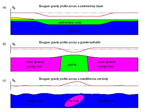
a) density of sedimentary rock < basement >> gravity low

b) density of granite less than rock >> gravity low

c) density of ore > rock >> gravity high

At sea, free-air gravity is generally used (measuring points in surface ships being generally at sea level), although sometimes a Bouguer correction is made by infilling the sea with imaginary rock.

Bouguer gravity in the oceans is normally high, because the mantle surface (MOHO) is at shallow depths, but free-air gravity is low because the oceans are in isostatic equilibrium.

Satellite-derived free-air gravity map of Sandwell and Smith (Nature, 1997) for the North Atlantic Ocean.

Red/yellow colours indicate gravity highs and purple/blue colours indicate gravity lows. The large white circle on Iceland indicates the location of the present-day plume centre at Vatnajökull (64.5° N, 17.3° W). Up to 500 km southwest along the Reykjanes ridge spreading centre, indicated by the solid white line, asthenospheric potential temperatures of 1,450 °C result in the generation of a 14-km-thick oceanic crust. Filled circles delineate prominent V-shaped ridges which transgress the magnetic anomaly pattern. These ridges are symmetrical about the spreading axis and converge southwards thus crossing progressively younger crustal isochrons.

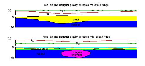
The mountain range and mid-ocean ridge are in isostatic equilibrium, so the free-air gravity profiles are virtually flat. The Bouger profiles show gravity lows due to the low-density mountain roots in (a) and from the low density magma chamber in (b) (of the order of -300 g.u. and -1000 g.u respectively).

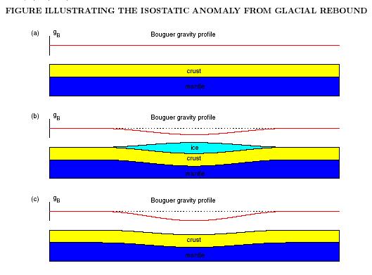
The reality of isostasy is confirmed by the measurable uplift of Fennoscandia during the last two hundred years as a consequence of the unloading accompanying the melting of the ice sheets. Below the figure shows a) the crust in isostatic equilibrium before the ice-age, b) loading of the crust by an ice-cap, and c) the rebounding crust after the ice has melted. In b) the crust sags, forming a root that supports the ice cap; the mantle material flows away from the depression. The root causes a negative Bouger anomaly. When the ice melts the crust starts to rebound and the mantle material flows back into the region. The viscosity of the mantle is the controlling factor in the rate of rebound. Mantle viscosities can be estimated from rates of glacial rebound

But not all structures are in isostatic equilibrium. The Hawaiian chain is such an example where the free-air gravity map shows highs in line with the topography, which would not be expected from an isostatically compensated structure.

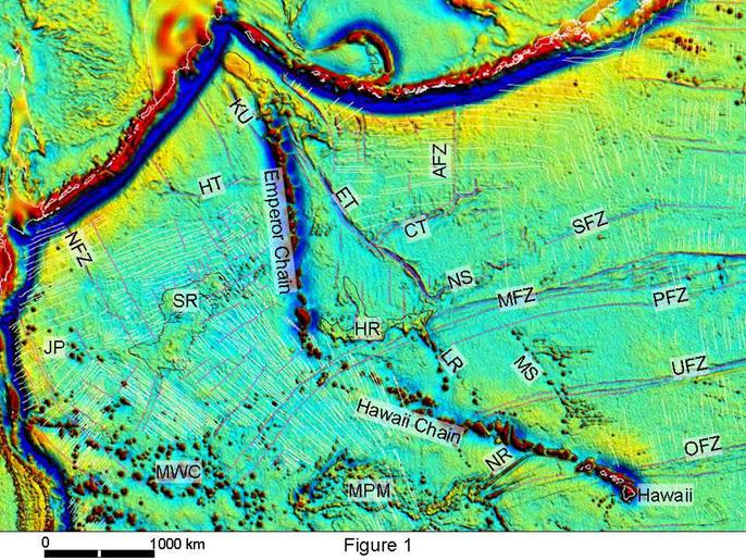
Free air gravity map of the northern Pacific showing Emperor-Hawaii seamount chain (Sandwell 13.1, 2005). Thin magenta lines are mapped fracture zones, thin yellow lines are identified magnetic lineations. SR = Shatsky Ridge; HR = Hess Rise; ET = Emperor Trough; CT = Chinook Trough; SFZ = Surveyor Fracture Zone; MFZ = Mendocino Fracture Zone; PFZ = Pioneer Fracture Zone; UFZ = Murray Fracture Zone; OFZ = Molokai Fracture Zone; AFZ = Amlia Fracture Zone; LR = Liliuokalani Ridge; MS = Musicians Seamounts; JP = Japanese Group seamounts; MWC = Marcus Wake chain; MPM = Mid Pacific Mountains; NFZ = Nosappu fracture zone; NR = Necker Ridge; KU = Kruzenstern fracture zone; NS = Non Surveyor feature, HT = Hokkaido Trough. Magnetic lineations (identified in Figure 2) are from compilatioms maintained by Larry Lawver and Lisa Gahagan at the Plates Project, Univerity of Texas at Austin, and my own updates digitized from Nakashini et al. (1989) and Atwater (1989). Mercator projection; scale bar is for approximately the latitude of Hess Rise.

Taken from Watts and Daly Ann. Rev. Earth Planet. Sci., 1981

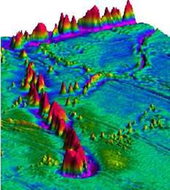
The sketch below shows the free-air and Bouguer anomaly associated with Hawaii both as derived from the observations, and also what the gravity observation would show if Hawaii were in isostatic equilibrium.

It is the gravity observation that tells us the coarse sub-surface structure of the shallow Earth.

Pratt and Airy Hypotheses

Gravity observations cannot tell us what the structures are like within the Earth, only whether or not there is a density excess or defecit. Two hypotheses exist which attempt to explain the gravity observations. That of Airy (below left) assumes that the rigid upper layer has a constant density that is lower than the substratum beneath. The mountain “floats” with deep roots like an iceberg. Conversely, Pratt (below right) assumes that the base of the upper layer is level, and it is the density within the upper layer that changes. Determining which of these hypotheses operates in the Earth is far from straightforward; however, in combination with seismology, detailed structures can be observed and understood.

Moment of Inertia

Circular motion

Just as linear velocity is distance travelled per unit time, so too angular velocity of a rotating body is the angle rotated per unit time. The angular velocity, ω, of a body rotating in a circular of radius r, with linear speed v, is:

ω = v/r

where ω must be in radians per unit time, normally, radians/s or rads/s.

Centripetal acceleration

Velocity is a vector and therefore is defined by both magnitude (speed) and direction. A rotating body is therefore changing its velocity continuously as it is always changing direction. It therefore has an acceleration. A body rotation on a circle of radius r, with linear speed v is being continuously accelerated towards the centre of the circle with a magnitude:

a = r ω² = v ω = v²/r

where a is in units of m/s²

Mass of the Earth from an orbiting satellite (e.g., the Moon)

From Newton’s Law, a body moving with angular velocity, ω, in circular orbit of radius R about the Earth will have a centripetal acceleration towards the Earth of:

F = ma = mR ω²

The force provided by the gravitational attraction between the Earth and the satellite is:

F = GMm/R²

Equating the two gives:

M=R³ ω²/G

Moment of Inertia

The mechanics of the Earth’s rotation avout its axis introduces a quantity called the moment of inertia, which is the rotational mechanical analogue of mass. The moment of inertia of a point mass, m, rotating at a distance, r, about an axis is mr². The moment of inertia of a body rotating about an axis is the sum of all the point contributions of the moments of inertia of the single point masses, m_i, within the body, each at a distance r_i from the rotation axis:

I = ∑m_ir_i²

The value for the moment of inertia therefore depends on the mass distribution within the body. For example, a bicycle wheel with all the mass concentrated on the rim would have a moment of inertia of mr²; if the mass was all in the axle, the moment of inertia would be zero; if the mass was evenly distributed across the wheel, I = 0.5mr².

In general, the moment of inertia is given by:

I = kmr²

Where k is a dimensionless constant that is object/material dependent. Examples include:

k = 1 a ring or thin walled cylinder rotating about its centre

k = 0.4 a solid sphere rotating about its centre

k = 0.5 a solid cylinder or disk rotating about its centre

For a sphere made up of homogeneous layers, the moment of inertia can be determined additively; for example, an Earth of radius R with a metal core of radius r and a silicate mantle:

metal

I_E = I_M(R) – I_M(r) + I_C(r)

= - +

silicate metal

Silicate silicate

See First Coursework Exercise

See Second Coursework Exercise

Useful websites

http://www.ngdc.noaa.gov/mgg/announcements/announce_predict.html

http://www.jpl.nasa.gov/earth/features/watkins.html

http://www.csr.utexas.edu/grace/gallery/animations/ggm01/index.html

Back to Contents